
|
|
COS 429 - Computer Vision |
Fall 2016 |
| Course home | Outline and Lecture Notes | Assignments |
 Dalal-Triggs:
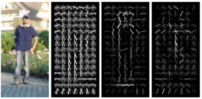
The 2005 paper by Dalal and Triggs
proposes to perform pedestrian detection by training a classifier on
a Histogram of Gradients (HoG), then applying that classifier throughout
an image. Your next task is to train that classifier, and test how well
it works.
Dalal-Triggs:
The 2005 paper by Dalal and Triggs
proposes to perform pedestrian detection by training a classifier on
a Histogram of Gradients (HoG), then applying that classifier throughout
an image. Your next task is to train that classifier, and test how well
it works.
Training: At training time, you will need two sets of images: ones containing faces and ones containing nonfaces. The set of faces provided to you comes from the Caltech 10,000 Web Faces dataset. The dataset has been trimmed to 6,000 faces, by eliminating images that are not large or frontal enough. Then, each image is cropped to just the face, and is resized to a uniform 36x36 pixels. All of these images are grayscale.
The non-face images come from from Wu et al. and the SUN scene database. You'll need to a bit more work to use these, though, since they come in a variety of sizes and include entire scenes. So, you will need to randomly sample patches from these images, and resize each patch to be the same 36x36 pixels as the face dataset.
Once you have your positive and negative examples (faces and nonfaces, respectively), you'll compute the HoG descriptor (an implementation of which is provided for you) on each one. Finally, you'll train the logistic regression classifier you wrote in Part I to run on the feature vectors.
As mentioned in the Dalal and Triggs paper and in class, the HoG descriptor has a number of parameters that affect its performance. Two of these are exposed to you, namely the number of orientations in each bin and whether those orientations cover the full 360 degrees or whether orientations 180 degrees apart are collapsed together. You will experiment with these parameters to see whether the conclusions reached in the paper (i.e., performance does not improve beyond about 9 orientations, and it doesn't matter whether or not you wrap at 180 degrees) hold equally well for face detection as for pedestrian detection.
 Predicting:
One of the nice things about logistic regression is that its output ranges
from 0 to 1, and is naturally interpreted as a probability. (In fact,
using logistic regression is equivalent to assuming that the two classes are
distributed according to Gaussian models with different means but the same
variance.) In Part I, you thresholded the output of the learned model to
get a 0/1 prediction for the class, which effectively thresholded at
a probability of 0.5. But for face detection you may wish to bias the
detector to give fewer false positives (i.e., be less likely to mark
non-faces as faces) or fewer false negatives (i.e., be less likely to mark
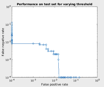
faces as non-faces). Therefore, you will look at graphs that plot the
false-negative rate vs. false-positive rate as the threshold of
probability is changed. Curves that lie closer to the bottom-left corner
indicate better performance. Of course, you will look at performance on both
the training set (for which you expect great performance) and a separate
test set (which may or may not perform as well).
Predicting:
One of the nice things about logistic regression is that its output ranges
from 0 to 1, and is naturally interpreted as a probability. (In fact,
using logistic regression is equivalent to assuming that the two classes are
distributed according to Gaussian models with different means but the same
variance.) In Part I, you thresholded the output of the learned model to
get a 0/1 prediction for the class, which effectively thresholded at
a probability of 0.5. But for face detection you may wish to bias the
detector to give fewer false positives (i.e., be less likely to mark
non-faces as faces) or fewer false negatives (i.e., be less likely to mark
faces as non-faces). Therefore, you will look at graphs that plot the
false-negative rate vs. false-positive rate as the threshold of
probability is changed. Curves that lie closer to the bottom-left corner
indicate better performance. Of course, you will look at performance on both
the training set (for which you expect great performance) and a separate
test set (which may or may not perform as well).
Do this:
Download the starter code and dataset
(about 30 MB) for this part. It contains the following files:
Once you download the code, copy over logistic_fit.m from part I. Then implement logistic_prob, get_training_data, and get_testing_data. Look for sections marked "Fill in here". The trickiest part is likely to be selecting random squares (i.e., random positions and random sizes no smaller than 36x36) from the nonface images.
Now run
test_face_classifier(250,100,4,true)
which trains the classifier on 250 faces and 250 nonfaces, tests it on 100 faces and 100 nonfaces, using 4 orientations that are wrapped at 180 degrees. If all goes well, the training should complete in a few seconds, and you should see two plots, for training and testing performance. The training plot should be boring: running down the bottom and left sides of the graph, indicating perfect performance. The testing plot, though, should indicate imperfect performance.Once you have your implementation working, experiment with the number of training images running up to 6,000, the number of testing images at 500, varying the number of orientations, and turning off the wrapping at 180 degrees. The training time may take longer and longer in this case, but should still finish in a few minutes, depending on your CPU.
Save and submit the false negative / false positive graphs for one set of parameters.
Answer and submit the following questions:
Acknowledgment: idea and datasets courtesy James Hays.
His
assignment at Georgia Tech.