COS 326

Assignment 7: Parallel Sequences

Quick Links

• Code Bundle for this assignment
• Preliminaries
• Web indexing
• US Census Population
• Hand-in Instructions
• Acknowledgments

Introduction

In this assignment, you will use the functional map-reduce abstraction to program two "big data" applications: search engine indexing and geographic information queries. Parallel functional map-reduce is used in the real world because of its efficiency and fault-tolerance in big server farms.

You may do this assignment in pairs. If you do so, both students are responsible for all components of the assignment. You should form a group to submit on TigerFile, which will allow both members of the pair to submit, but be careful about versioning: we will not be sympathetic to plights of having the wrong partner's version submitted.

Preliminaries

Type any of the following commands at the prompt to build components of the assignment:

  make seq       // Part 0 and Part 3: unit-testing the sequence library
  make idx       // Part 1: testing your inverted index construction
  make qpop      // Part 2: testing your population queries

One difference to note from previous assignments: our Makefile builds .native files (native machine code) rather than .byte files (portable bytecode for the OCaml bytecode interpreter). This makes the code go faster.

Since you probably don't have your own server farm, what to do? Actually, it's easy and cheap to rent a server farm, but we will do something else instead: use dynamic instrumentation to estimate the parallelism of your program. The Accounting functor instruments a Sequence implementation to measure work and span of the map-reduce programs you run. Your grade will depend, in part, on reducing the span of your algorithms (without increasing the work too much).

Caveat 1: When you perform map or reduce or scan (etc.) using your own ML functions f, g, etc., the automatic instrumentation does not measure the cost of f or g (except when they themselves do map-reduce operations). Therefore you must take care to avoid doing lengthy sequential computations inside the functions you pass to the map-reduce operators.

Caveat 2: Measurements of work versus span are not necessarily an accurate prediction of how fast your code would run on a big server farm.

Sequence library

The file sequence.ml (with interface sequence.mli) contains the module type S of sequences. You can see how work and span are estimated by inspecting module Accounting.

Caveat: After using seq_of_array arr to convert an array arr to a sequence, do not modify arr.

Caveat: After using let arr = array_of_seq s to convert a sequence to an array, do not modify arr.

The following table summarizes the most important operations in the sequence module and their work and span complexity.

Function	Description	Work	Span
tabulate	Create a sequence of length n where each element i holds the value f(i)	n	1
seq_of_array	Create a sequence from an array	1	1
array_of_seq	Create an array from a sequence	1	1
iter	Iterate through the sequence applying function f on each element in order. Useful for debugging	n	n
length	Return the length of the sequence	1	1
empty	Return the empty sequence	1	1
cons	Return a new sequence like the old one, but with a new element at the beginning of the sequence	n	1
singleton	Return the sequence with a single element	1	1
append	Append two sequences together. append [a0;...;am] [b0;...;bn] = [a0;...;am;b0;...;bn]	m+n	1
nth	Get the nth value in the sequence. Indexing is zero-based.	1	1
map	Map the function f over a sequence	n	1
reduce	Fold a function f over the sequence. To do this in parallel, we require that f has type: 'a -> 'a -> 'a. Additionally, f must be associative	n	log(n)
mapreduce	Combine the map and reduce operations.	n	log(n)
flatten	Flatten a sequence of sequences into a single sequence. flatten [[a0;a1]; [a2;a3]] = [a0;a1;a2;a3]	n	log(n)
repeat	Create a new sequence of length n that contains only the element provided repeat a 4 = [a;a;a;a]	n	1
zip	Given a pair of sequences, return a sequence of pairs by drawing a value from both sequences at each shared index. If one sequence is longer than the other, then only zip up to the last element in the shorter sequence. zip [a0;a1] [b0;b1;b2] = [(a0,b0);(a1,b1)]	n	1
split	Split a sequence at a given index and return a pair of sequences. The value at the index should go in the second sequence. split [a0;a1;a2;a3] 1 = ([a0],[a1;a2;a3]) This routine should fail if the index is beyond the limit of the sequence.	1	1
scan	This is a variation of the parallel prefix scan shown in class. For a sequence [a0; a1; a2; ...], the result of scan will be: [f base a0; f (f base a0) a1; f (f (f base a0) a1) a2; ...]	n	log(n)

Part 1: An Inverted Index Application

The following application is designed to exercise the "Map-Reduce" style of computation, as described in Google's influential paper on their distributed Map-Reduce framework.

When implementing your index, you should do so under the assumption that your code will be executed on a parallel machine with many cores. You should also assume that you are computing over a large amount of data (e.g.: computing your inverted index may involve processing many documents). Hence, an implementation that iterates in sequence over all documents will be considered impossibly slow — you must use bulk parallel operations such as map and reduce when processing sets of documents to minimize the span of your computation. Style and clarity is important too, particularly to aid in your own debugging.

As you develop your algorithms (for all parts of this assignment), you should measure their work and span. After you import and open the Sequence module, suppose you write a function f: t1 -> t2 that uses use operations S.tabulate, S.map, et cetera. You can measure work and span by invoking Acc.reporting "measuring:f" f x which calls f(x) while measuring work and span, and produces a line like,

measuring:f w=256 span=109

Part 1a: Inverted Index

An inverted index is a mapping from words to the document and location within the document in which they appear. Read 9 Algorithms that Changed the World chapter 2: "Search Engine Indexing", available on reserve for this course (log into blackboard.princeton.edu for COS 326). For example, if we started with the following documents: Document 0:

OCaml, map reduce

Document 1:

::fold filter ocaml

The inverted index would look like this:

word	document
ocaml	0:0:0 1:2:14
map	0:1:7
reduce	0:2:11
fold	1:0:2
filter	1:1:7

For each word, there is a sequence of doc-number:word-number:char-number pairs. For example, "ocaml" is in document 0 at word 0 (character position 0), and in document 1 at word 2 (character position 14). To implement this type of index, complete the make_index function in inverted_index.ml. This function should accept a sequence of documents, and return the index. The data file is a condensed set of documents (such as the three data/test_index_*.txt files provided), one per line. Each document record has an id number, a title, and the document's contents. To get started, investigate some of the functions in the module Util (with interface util.mli and implementation util.ml). In particular, notice that Util contains a useful function called load_documents: use it to load a collection of documents from a file.

Attention to detail: The example above suggests that your inverted index should be case insensitive (OCaml and ocaml are considered the same word). You might find String.lowercase_ascii from the String library useful.

Part 1b: Phrase search

As explained in 9 Algorithms that Changed the World, having the location-within-document allows queries such as "foo near bar", meaning, "find documents where "foo" appears within k words of "bar".

We will do something related: look for a string such as "for a year". That is, find all documents where the word "for" is the ith word, for some i, and then the (i+1)th word is "a" and the (i+2)nd word is "year". Implement a function search that takes an index and a query (a list of strings) and returns a list of results. A result has a document-number, a begin-character-position of the phrase in that document, and an end-character-position. (To keep things simple, let the end-character-position be the position of the first character in the last word of the phrase.)

Testing

We have provided main_index.ml, which is a driver that calls your function to build an index from a given file, then (if you use the -dump option) prints the resulting index out in string form. To run, first compile into an executable for testing with the given Makefile using make idx. Then run the main_index.native program with its first command line argument being the datafile. Here's an example:

./main_index.native -dump data/test_index_1.txt 
Key: {'one'} Values: {'1:4', '1:3', '1:2', '1:1'}

Command-line arguments after the name-of-index-file are treated as a search query; for example,

./main_index.native data/test_index_1000.txt for a year
940: t rise in December, for a year-on-year rise of
908: ts to 96,000 tonnes for a year from March 1.  
382: d not pay principal for a year and a half, the
16: il pays no interest for a year, said Joseph Ar
4: il pays no interest for a year, said Joseph Ar

DO NOT change any of the types or functors provided for you — these must match the given interface. You may write additional functions so long as you do not require them to be visible outside the module.

To submit for Part 1: inverted_index.ml

Part 2: US Census Population

The goal for this part of the assignment is to answer queries about U.S. census data from 2010. The CenPop2010.txt file in the data directory contains data for the population of roughly 220,000 geographic areas in the United States called census block groups. Each line in the file lists the latitude, longitude, and population for one such group. For the sake of simplicity, you can assume that every person counted in each group lives at the same exact latitude and longitude specified for that group.

Suppose we want to find the total population of a region in the United States. How might we go about doing this? Since we can approximate the area of any shape with sufficiently many rectangles, we will focus on the simpler problem of efficiently finding the population for any rectangular area. We can think of the entire U.S. as a rectangle bounded by the minimum and maximum latitude/longitude of all the census-block-groups — this includes all of Alaska, Hawaii, Puerto Rico, and parts of Canada and the ocean. We might want to answer queries related to rectangular areas inside the U.S. such as:

• For some rectangle inside the U.S. rectangle, what is the 2010 census population total?
• For some rectangle inside the U.S. rectangle, what percentage of the total 2010 census U.S. population is in it?

We will investigate two different ways to answer queries such as these: 1) the query search method: a slower, simpler implementation that looks through every census group in parallel, and 2) the precomputation method: a more efficient implementation that precomputes intermediate population sums to answer queries in constant time.

Query Search

We can answer a population query by searching through all the census groups and summing up the population of each census group that falls within the query rectangle. This naïve approach must look through every single census group. However, using our parallel sequence implementation, we can mitigate this exhaustive technique by looking through census groups in parallel.

We have implemented the search-based population query in the query.ml file for you. This will serve as a reference implementation that you can use to verify your results for the precomputation-based part of the assignment that follows.

Query Precomputation

Looking at every census group each time we want to answer a query is still less than ideal, even in parallel. With a little extra work up front, we can answer answer queries more efficiently. We will build a data structure called a summed area table in order to answer queries in O(1) time.

Conceptually, we will overlay a grid on top of the U.S. with x columns and y rows. This is what the GUI we provide is showing you (see GUI description below). We can represent this grid of size x*y as a sequence of sequences, where each element is an int that will hold the total population for all positions that are farther South and West of that grid position. In other words, grid element g stores the total population in the rectangle whose bottom-left is the South-West corner of the country and whose upper-right corner is g. (This should be reminiscent of prefix-sum.)

Once we have this grid initialized, there is a neat arithmetic trick to answer queries in O(1) time. To find the total population in an area with lower-left corner (x1,y1) and upper-right corner (x2,y2), we can take the value for the top-right corner, and subtract out the values at the bottom-right and top-left corners. This leaves just the area we want, however, we have subtracted the population corresponding to the bottom-left corner twice, so we must add it back once more.

For this part, you must build a summed area table and answer queries by consulting the table. You should create the summed area table as follows:

1. Start by initializing the grid with each element corresponding to the population just for census groups in that grid element.
2. Next, build the final summed area table using appropriate operations from the parallel sequence library.

You will implement the precompute and population_lookup functions in query.ml. You can now test your results by following the instructions in the Testing and Visualization section below. Your results from the search-based population query and the precomputation-based population query should match.

Testing and Visualization

We have provided the parse.ml and population.ml files to read the census data and answer queries via command line arguments passed to the program. The format for a query is:

./population.native [file] [rows] [cols] [left] [bottom] [right] [top]

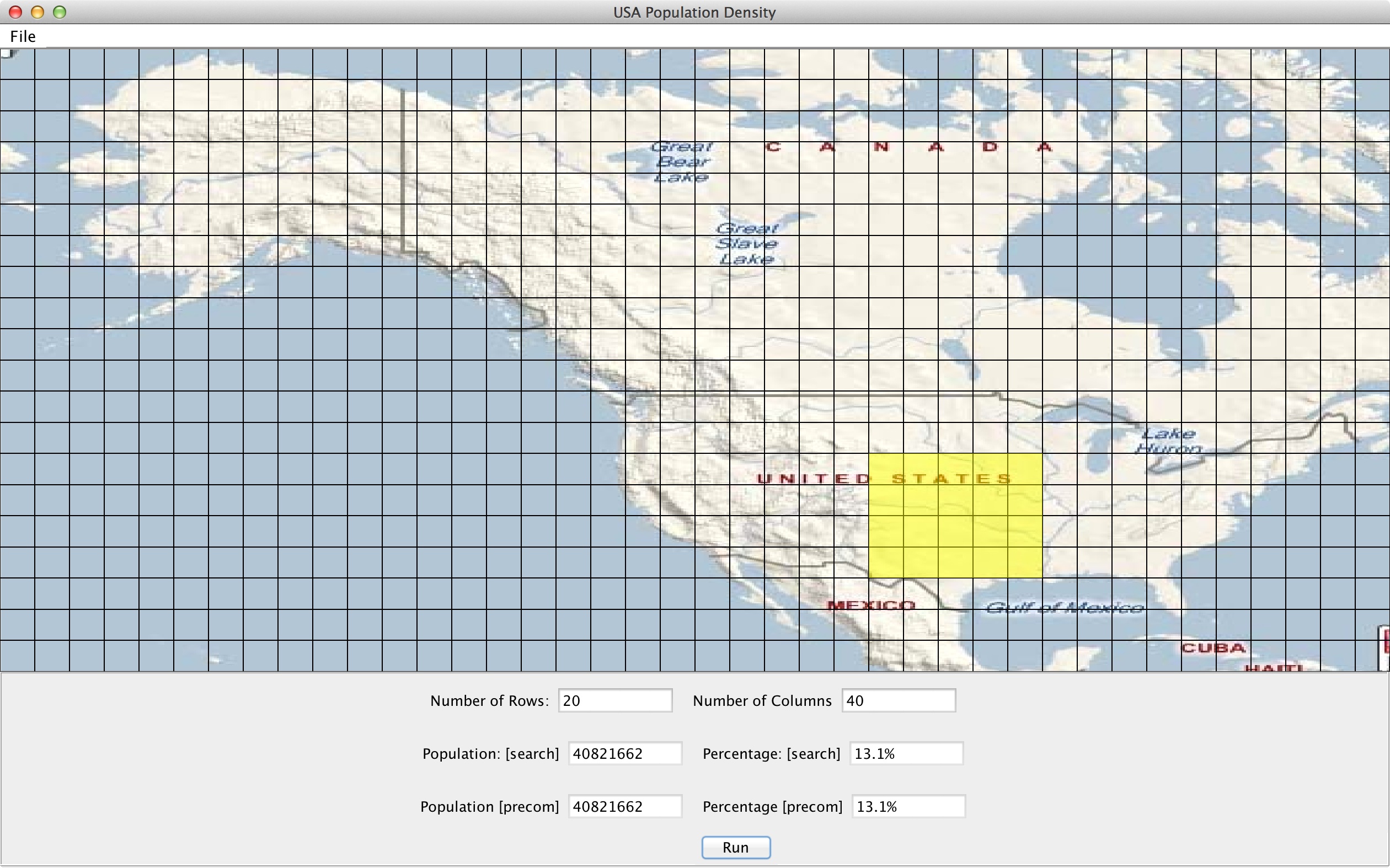
The number of rows and columns are used for summed area table. Left, bottom, right, and top describe the row and column grid indices (starting at 1) that define the rectangular query. For example, to query a the section of the central U.S. shown highlighted in the picture below using a 20 row 40 column grid, you would run the following command:

./population.native data/CenPop2010.txt 20 40 26 4 30 7
40821662,13.1
40821662,13.1

The program will evaluate the query using both the implementations described above and list the total population and percent of the U.S. population for both. To make testing easier, we provide a GUI that displays a map of the U.S. that you can interact with. You can change the number of rows and columns, select a region on the map, and ask the GUI to run your program to display the answer.

java -jar USMap.jar

To help you debug your code, there are a number of example queries and results listed below. Your answer should roughly match up with the search-based implementation. It is okay if you get slightly different answers (depending on how you handle edge cases), but make sure that you are at least accurate to the nearest percent.

# Population of the western half of the United States
./population.native data/CenPop2010.txt 10 10 1 1 6 10
64620478,20.7
64620478,20.7

# Population of the mainland United States
./population.native data/CenPop2010.txt 100 200 89 8 191 45
305896552,97.9
305896552,97.9

# Population of Alaska
./population.native data/CenPop2010.txt 2 1 1 2 1 2
710231,0.2
710231,0.2

To submit for Part 2: query.ml

Part 3: Associativity

Inspect sequence.ml, especially in the module ArraySeq the implementation of map_reduce and reduce. Notice that these are entirely sequential implementations that apply the function g left to right. But a parallel implementation would apply g in a tree-like divide-and-conquer. This will yield the same result if g is associative and base is a unit for g.

Are you sure that every time you used map_reduce or reduce or scan your function was associative and your base was a unit for it? How would you even prove that? (Oh, wait a second, we know how to prove it. But instead...) Here's a way of experimentally testing that question.

In the module ArraySeqAlt, replace the line let map_reduce = ArraySeq.map_reduce with a divide-and-conquer implementation. (ArraySeq.t is opaque, but you can implement this entirely as a client of the abstraction, using S.split.)

Then run your programs using ArraySeqAlt in place of ArraySeq, by modifying the 2nd-to-last line of sequence.ml. Do you get the same results?

To submit for Part 3: sequence.ml

Performance analysis

In the section of your README that says, "Report your work and span numbers", fill in the ? with your actual numbers.

Then, in the section "Analyze your work and span numbers",

• Define the problem size, N (total size of the actual input to make_index or precompute)
• As a function of N, based on the measured work and span, and based on the algorithms you are using, estimate the asymptotic complexity of the work and span of each of these three functions. Is it quadratic, NlogN, linear, logN, (logN)^2, etc. ?

As you know if you took COS 226, this kind of estimate is more meaningful if you measure on inputs of several different sizes and make a graph, but here it might be OK to eyeball it from just one N.

Handin Instructions

You must hand in these files to TigerFile (see link on assignment page):

1. README.txt
2. sequence.ml
3. inverted_index.ml
4. query.ml

Acknowledgments

This assignment is based on materials developed by Dan Licata, David Bindel, and Dan Grossman, further developed by Nate Foster, Ryan Newton, Christopher Moretti, and Andrew W. Appel.

Princeton University, Computer Science Department
Template design Andreas Viklund