COS 429 - Computer Vision

Fall 2017

Assignment 0: Setup

1. Getting familiar with Matlab

Princeton has a site license of Matlab, and you should install it on your own machine - instructions are here.

Read through the following for a basic introduction to Matlab:

• A short Matlab introduction
• The demos accessible by typing "demo" within Matlab.

Work through the following tasks using an image of your choice:

1. Read an image into a variable.
   Hint #1: "help imread"
   Hint #2: Use single quotes around the filename.
   Hint #3: Ending a command with a semicolon supresses printing the result.
   
   
2. Display the image.
   Hint: "help imshow"
   
   
3. Convert the image to grayscale.
   Hint: "help rgb2gray"

   Note: if your version of Matlab doesn't have the rgb2gray function, download rgb2gray.m. Place this in your working directory, and it should be auto-loaded by Matlab.

4. Convert the grayscale image to floating point.
   Hint #1: "help im2double", and be aware of the difference between im2double(img) and double(img).
   Hint #2: imshow is able to also display floating-point images.
   
   
5. Plot the intensities along one row of the grayscale image.
   Hint #1: Extracting a part of a matrix is done by

   	matrix2 = matrix1(row_min:row_max,col_min:col_max);
   

   The indices are inclusive: array(low,high) returns the set [low, high].
   row_max or col_max may also be "end" to indicate the last element.
   Just a ":" is equivalent to "1:end".
   Hint #2: BIG WARNING: indices in Matlab are 1-based (not 0-based as in C or Java).
   Hint #3: "help plot"
   
   
6. Store the width and height of the image in variables "width" and "height".
   Hint #1: "help size"
   Hint #2: Functions in Matlab may return multiple values. You can get at the values using the notation

   	[var1, var2] = func(x)
   

   Hint #3: In Matlab, the number of rows is the first dimension and the number of columns is the second. In terms of an x,y coordinate scheme, (row, col) indexing means images have shape [height, width] and can be indexed as image(y, x).
   
   
7. Write a pair of nested "for" loops to set a grid of every 10th pixel horizontally and every 20th pixel vertically to 0.
   Hint #1: "help for"
   Hint #2: "start:increment:stop"
   
   
8. Create a function "maxrow" that takes a matrix and a row index and returns the brightest pixel in the given row. Store the function in a file called "maxrow.m" so that Matlab loads it automatically when you call the function.
   Hint #1: "help function"
   Hint #2: "help max". Matlab has many built-in functions that operate on entire vectors or matrices, and using those is usually much, much more efficient than writing a "for" loop.
   
   
9. Flip an image vertically. Then show the original and the flipped image side-by-side.
   Hint: "help subplot"
   
   
10. Write the modified image back to a new file.
    Hint #1: "help imwrite"
    Hint #2: For RGB images imwrite supports both uint8 and floating point pixels. For floating point images, the valid range of values is [0.0, 1.0].
    
    

If you get stuck on any of these, ask for help on piazza.

2. Getting MatConvNet up and running

1. Follow the MatConvNet installation instructions. Feel free to skip the DAG models section. In this class we will be training only smaller networks where the CPU-only implementation should be sufficient. If you happen to have an NVIDIA GPU in your machine and have the CUDA development libraries installed, feel free to set up the GPU training as well. When done you should see:
   
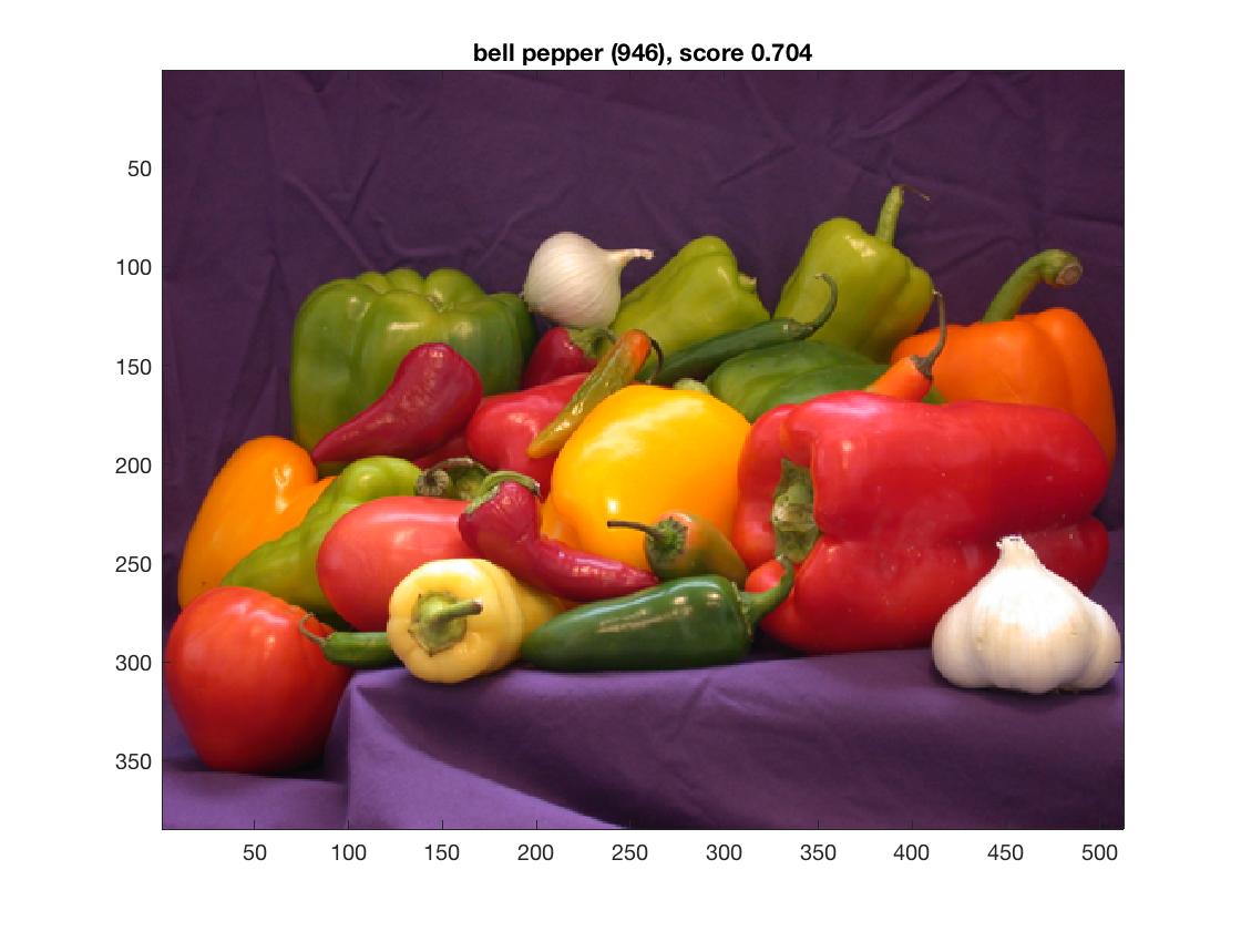
2. Run the classification network on other images. Where does it work surprisingly well? Where does it make mistakes?