Projecting Color onto Michelangelo's Statues

Szymon Rusinkiewicz

This webpage documents the color processing pipeline used in the Digital Michelangelo Project to derive surface color for Michelangelo's sculptures.

1. Motivation

Q: Why bother? Aren't marble sculptures basically all white?

A: No, the sculptures are not all white. There are many sources of (subtle) coloration:

• Natural variations in the color of the marble, veining
• Chisel marks, which crush the marble
• Dirt, dust, grime
• Waxes and other surface polishing agents
• Weathering and erosion, if the statue has stood outside (e.g. David)
• Wearing due to human contact

• The presence of dirt or wax on a statue give important clues to a statue's history. The David is especially interesting in this regard, since he stood outside for hundreds of years before being moved indoors to the Accademia. Certain areas show pronounced weathering, and their exact nature provides some insight into the preservation and restoration attempts that have been made over the centuries.
• Evidence of human contact is clearly useful in determining how the statue has changed since Michelangelo's time, and in evaluating possible restoration.
• The very finest chisel marks are less than 100 microns deep. Because of the noise inherent in our range measurements, these chisel marks show up more clearly in the color data than our range data.

Since it is our goal to make definitive archival computer models of the statues, it is important that we document all of these effects.

Q: Isn't it trivial to get color? Can't you just take a bunch of pictures and use them as texture maps?

A: Using individual pictures as texture maps would work only if we wanted to re-render the mesh from the same camera position and under the same lighting conditions as were present when the pictures were taken. We want to go much further - we want to be able to generate photorealistic renderings of the mesh from arbitrary viewpoints and under arbitrary lighting conditions. To do this we need the actual reflectance at each point on the surface. In particular, for each image we need to separate the effects of surface reflectance from the effects of lighting. We are able to do this by using a combining a calibrated camera and lightsource with our high-resolution geometry.

2. Hardware

Our color data comes from four sources:

1. A Sony DKC-5000 mounted permanently in the scanhead of our Cyberware statue scanner. This is a 3-CCD digital camera with a resolution of 1520x1144. We have also mounted a 250W fiber optic white light source at a known position in the scanhead, and have calibrated the position and orientation of the camera and light relative to the laser and range camera.
2. A second DKC-5000 and 250W lightsource mounted on a Faro Arm. This scanner can be interchanged with a ModelMaker scanner that also mounts on the Faro Arm, and we can calibrate the position and orientation of the camera in the space of the range data returned by the ModelMaker.
3. A Sony DKC-ST5 mounted to our Cyrax scanner. This is a higher-resolution 3-CCD digital camera, with an image resolution of 2048x2560. Because we use the Cyrax to scan large architectural spaces and do not have a calibrated light source useable over such large distances, we cannot derive surface reflectance from these images and use them only for texture mapping.
4. The Sony DKC-ST5 used alone, with either white light or ultraviolet lighting.

In each case, we calibrate the intrinsic properties (focal length, geometric distortion, chromatic aberration, vignetting, etc.) of the camera/lens combination, and use that data to correct the images before projecting them onto our meshes.

3. Processing

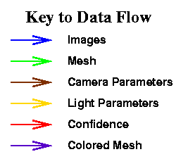
Here is an overview of the image processing pipeline:

"Ambient" vs. "lit" pictures

The first thing to notice is that this pipeline starts with not one but two images. The reason for this is simple - in order to separate the effects of surface reflectance and lighting in each picture, we have to know the complete the complete geometry and lighting of the rooms around these statues. Since this is something we typically do not and cannot know, and since it is impractical to turn off all the room lights during scanning we cannot assume that the only light contribution to the pictures we take is our light. To get around this problem, we use the following trick: we take two complete sets of pictures from identical camera positions. For each position, the first picture is taken using only the "ambient" lighting of the room, and the second includes both this ambient lighting and our own, calibrated, light source. Then, we just subtract the first picture from the second. In this way, we obtain a picture showing what the camera would have seen if the only light had come from our light source.

Correcting and merging images

The next steps in the color processing pipeline are to correct the images to undo systematic camera distortion, undo the effects of lighting, and project the color onto the mesh. We cover these steps in detail below. The result of the steps is a mesh that has been colored by one image - each vertex has red, green, and blue surface reflectance as computed from that image as well as a confidence that indicates how much we trust those results. Since it is typically the case that we have more than one image that saw each point on the surface, the final step in our pipeline is to merge the estimates of surface color from the different images.

The merging step proceeds by looking at the confidences assigned to each point from each image. Clearly, the image that had the greatest confidence in its estimation of the color of a given vertex should be given the greatest weight in the final color of that vertex. In order to avoid visible seams, however, the other estimates of the color of that vertex should also be included in the final color, so that the final output color blends smoothly between the different images. In doing this blending, however, we must be careful to include only relatively high-confidence estimates: if we have a low confidence estimate than its inclusion, even with a relatively low weight, could leave significant artifacts in the data.

For example, one of the motivations for lowering the confidence of our data is if we suspect that the image contains a specular highlight. If we were to blend good data with data contaminated with such a specular highlight, then the highlight might show up, to some extent, in the final estimated color. To avoid this, we look for the highest-confidence estimate of color at each vertex, and only blend among those estimates with confidence at least half of that maximum - estimates with lower confidence are discarded completely. In this way, we arrive at a final estimate of color for each vertex in the mesh.

Let us now take a closer look at the box labeled "Correct and Project" in the above diagram:

Camera lens distortion correction

No camera lens performs perfect perspective projection - there is always some amount of distortion. The most common and most pronounced is the familiar first-order radial "barrel" or "pincushion" distortion, but lenses can also exhibit higher-order radial or tangential distortion. As part of our calibration process we compute a geometric distortion model for our lens that includes two radial and two tangential distortion terms, off-center perspective projection, and a possibly non-uniform (in X and Y) scale. In addition, we determine the radiometric distortion of the lens/camera system - that is, the effects of lens vignetting and non-uniform sensor response on the images. This distortion model is used to correct the pictures at an early stage in our processing pipeline.

Sample distorted image	After geometric distortion correction

Image of a white card with radiometric distortion	After radiometric distortion correction

Chromatic aberration correction

The exact focal length, and hence the magnification, of a real lens depends on the wavelength of light. This phenomenon is known as chromatic aberration, and is most frequently seen as red and blue fringes around high-contrast regions, particularly near the edges of an image. Since our camera gives us only three "colors", each of which is actually an integration over many visible wavelengths, it is impossible to correct completely for the effects of chromatic aberration. Nevertheless, it is possible to correct partially by computing an average aberration for each of the red, green, and blue color channels. As part of our calibration process we determine these numbers for the lenses we use, and later use these parameters to correct our images.

Detail of image showing chromatic aberration	After chromatic aberration correction

Mesh visibility computation and projecting color

Once we have corrected our images, we are ready to project them onto the mesh of the statue. The first step in that process is to determine exactly which vertices in the mesh are visible from the given camera position, and which are visible from the light. This could be done using a raytracer, but for large meshes it is more efficient to use a hardware-accelerated shadow buffer algorithm. Essentially, we render the mesh from the point of view of the camera and light source with depth buffering enabled. We then read back the contents of the depth buffer, and compare the actual depth of each vertex to the contents of the depth buffer at the correct (x,y) position. If the depth buffer contained a smaller value, the vertex is not visible from the camera or light source. Once we know what is visible, we just project the coordinates of each vertex into the camera image, and sample the image at the computed (x,y) position.

Lighting correction

Once we have projected an image onto the mesh, we need to undo the effects of lighting, so that we are left with the intrinsic surface reflectance. The first part of this computation involves first dividing the color at a vertex by the cosine of the angle between the surface normal and the vector from the surface point to the light source. Note that this implicitly assumes that the surface is perfectly diffuse (i.e. has a Lambertian BRDF). This assumption is reasonable for most surfaces, especially if the camera image is looking "head on" at the surface. The second step in the correction involves adjusting for the irradiance of the light source at the surface - since the light source approximates a point light, this can be computed from the inverse-square law.

Let us now take a closer look at the confidence-processing pipeline:

Confidence from the projection stage

During the process of projecting images onto the mesh, we compute quantities like the orientation of the surface with respect to the camera and light. These are natural starting points for our confidence estimates - the more tilted (foreshortened) the surface is with respect to the light or camera, the lower our confidence of the surface reflectance at that point should be. Also at this stage, we can compute the potential locations of specular highlights and reduce confidence there.

Silhouette edges

Because of the integration over the area of a camera pixel and, more significantly, blur in the lens, the pixel values around occlusion edges and other depth discontinuities in the mesh will include color from both the occluding and occluded surfaces. For this reason, these color values should get reduced confidence. We accomplish this by looking for silhouette edges in the renderings of the mesh from the point of view of the camera and light, and reducing confidence in the regions close to these edges.

Saturated regions

If some pixels in one of the original images have been saturated, perhaps because of a specular highlight, we greatly reduce their confidence. Similarly, we reduce confidence in any areas of the original images that are particularly dim - they might be stray shadows that we failed to detect by other means.

Feathering confidence around edges

If we are to get truly seamless blends between images, we must ensure that there are no places where confidence suddenly changes drastically. The edge of the image is one such place, so we always reduce confidence around the edges of an image.

Combining and smoothing confidence

The confidence estimates from all the above sources are combined, then smoothed to avoid sharp transitions. The final confidences are used in the merging stage as described above.

4. Sample results

The following shows a few stages of the color processing pipeline applied to the St. Matthew:

A few notes:

1. All meshes are shown smooth shaded and re-lit with a single point light source.
2. Bright blue in colored meshes indicates missing color data.
3. You can click on any picture above to bring up a larger version.