How to Scale Hyperparameters as Batch Size Increases
Understanding Optimization using Stochastic Differential Equations
TL;DR: Stochastic differential equations (SDEs) provide rigorous, empirically validated scaling rules that prescribe how to adjust hyperparameters when scaling training runs (Adam or SGD, language or vision) to highly distributed settings without sacrificing performance. This post focuses on empirically useful insights, and a subsequent post will describe the theoretical toolbox of SDEs in more detail.
Scaling Rules: Increase Batch Size without Hurting Performance
Even as early as 2011, researchers recognized that scaling training runs across GPUs can yield huge efficiency gains (HOGWILD! by Niu et al.). For example, loading a large minibatch using data parallel with 8x as many GPUs allows you to finish training nearly 8x as fast (modulo communication and latency). However, using a very large batch size naively hurts SGD performance and puts a limit on how much you can scale (Keskar et al., 2017). A few papers subsequently suggested that one needs a scaling rule to adjust the hyperparameters when increasing the batch size. There are different scaling rules for different optimizers.
Linear Scaling Rule (for SGD)
When scaling the batch size by $\kappa$, scale the learning rate also by $\kappa$.
Square Root Scaling Rule (for Adam)
When scaling the batch size by $\kappa$, scale the learning rate by $\sqrt{\kappa}$. Also, change the other hyperparameters, setting $\beta_1 = 1 - \kappa(1-\beta_1)$, $\beta_2 = 1-\kappa(1-\beta_2)$, and $\epsilon = \epsilon / \sqrt{\kappa}$.
Even so, without rigorous theory, it was unknown what the maximal performant batch size was, so scaling runs up was an expensive trial-and-error game. In 2014, Krizhevsky heuristically derived a square root scaling rule for SGD, stating that the learning rate should be scaled by $\sqrt{\kappa}$ when scaling the batch size by $\kappa$ (see the bottom of page 5). This ends up being incorrect! Even Krizhevsky notes that the linear scaling rule yields empirically stronger performance. But later work in (Hoffer et al., 2017) agreed with the square root scaling rule.
At the same time, an empirical work trying to train a ResNet-50 on ImageNet in 1 hour (i.e., in a highly distributed setting), derived the linear scaling rule under the assumption that the gradient doesn’t change much during training (Goyal et al., 2017). Despite a few other optimization tricks, the test accuracy still degraded at large batch size. (Smith et al., 2020) also derived the linear scaling rule using reasoning analogous to a central limit theorem but still noted the batch size needs to be small for the rule to hold.
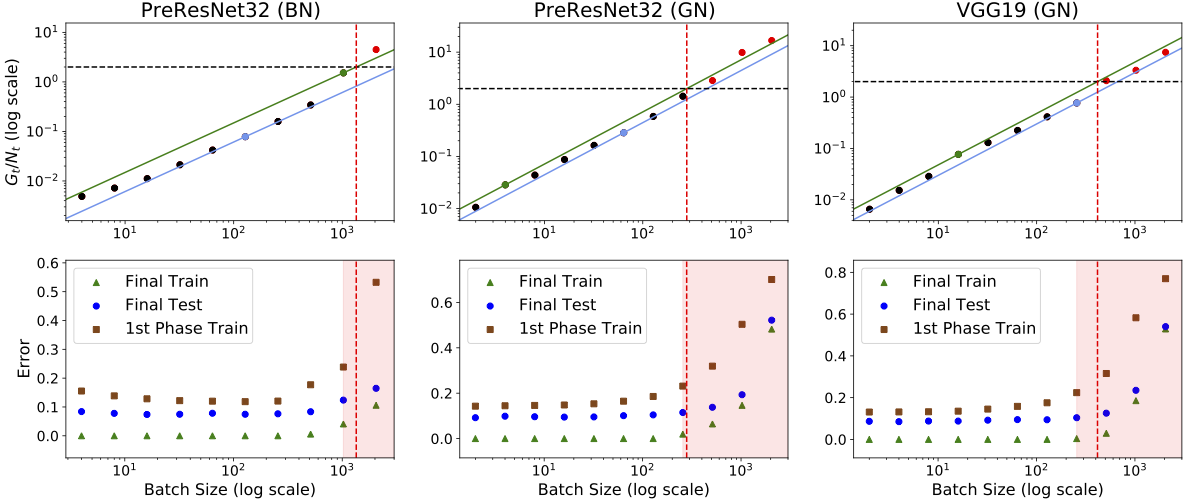
To clear up which scaling rule is correct and when it will break, we can turn to SDEs! Our work in NeurIPS 2021 used SDEs to design a simple test (requiring just one baseline run!) for the largest batch size you can parallelize to via the linear scaling rule without sacrificing performance. See the figure below. We also designed an efficient simulation of the SDE that provided evidence that the SDE is the correct way to model many realistic SGD training settings. (The next section explains why SDEs are so useful in analyzing SGD.)
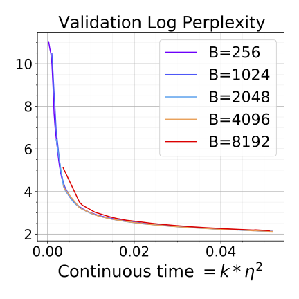
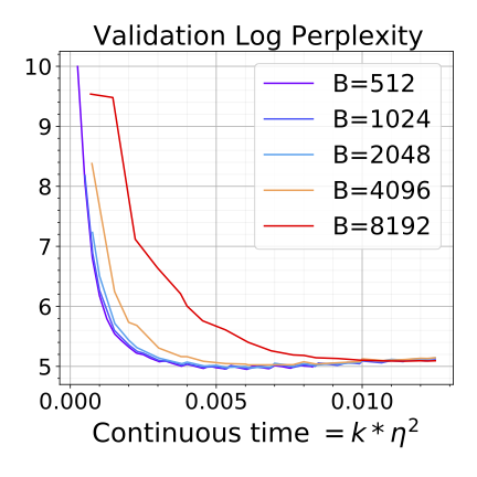
In the meantime, language models started to grow popular. (You et al., 2020) designed a scheme to train a BERT model in 76 minutes with Adam, and they empirically discovered that scaling the learning rate by $\sqrt{\kappa}$ works well. Our work in NeurIPS 2022 approached the question theoretically and established new SDE approximations for Adam and RMSprop. These yielded a square root scaling rule for Adam, which requires scaling the other optimization hyperparameters in addition to the learning rate. Experiments showed that the square root scaling rule preserved test accuracy, perplexity, and even post-fine-tuning performance. Naturally, these scaling rules will break at some large batch size, but we couldn’t find any empirical setting at the time where this happened.
Various works have since used the SDE approximation to derive useful distributed training protocols when using EMA (Busbridge et al., 2023) and Local SGD (Gu et al., 2023).
Into the Weeds with SDEs
Now that I’ve described the importance of SDEs, I’ll describe what they are exactly and how they can be used. SDEs describe a continuous trajectory of the model parameters over the course of training. The hypothesis is that this continuous trajectory is a reasonable and easily analyzable approximation of the discrete parameter trajectory that SGD prescribes. So let’s see how it shakes out.
At each step, SGD samples a minibatch $B_t\subset \mathcal{D}$ and updates the parameters according to some loss function $\ell$: $\theta_{t+1} = \theta_t - \eta\nabla \ell(B_t;\theta_t)$. Everyone knows the crucial hyperparameter $\eta$, the learning rate, but people often overlook the batch size hyperparameter, $B$, which is usually set to be the largest allowable value on the GPU (for pre-training) and carefully grid-searched (in fine-tuning). These two hyperparameters together control how much noise there is in the gradient estimate and how it affects the trajectory. The gradient noise is what makes SGD different from GD, so we will try to study this property carefully to understand why SGD results in better generalization than GD.
One approach to studying SGD is to use a continuous approximation of the discrete trajectory. This admits the derivation of results about the exploration and convergence of the optimization. One way to get a continuous approximation is to take the learning rate to be very small (i.e., $\eta\to 0$), which gets us to the famous gradient flow (GF) limit: $dX_t = -\nabla\ell(\mathcal{D};X_t)dt$. I’ll start to use $X$ to denote the continuous trajectory of the parameters and $\theta$ to denote the discrete one. GF used to be and still somewhat is the tool of choice to analyze how optimization proceeds. But if we look closely, we can see that GF is agnostic to the batch size! So, even if I was doing full-batch GD, I would still end up with GF as the limit. This means that GF can’t tell us much about the benefit of SGD over GD.
OK, so we need to find a continuous process that can actually model the gradient noise. This is where SDEs come in handy! Here’s the SDE used to approximate SGD (Li et al., 2019):
The first term of our SDE is the drift, the deterministic term in the process, which is just the full-batch gradient in this case. The second term is the diffusion, which we traditionally model using Brownian motion $W_t$. So, the SDE is actually very intuitive: we believe that SGD is doing something like GD + noise and we can clearly see that intuition in these two terms. Another key feature is that the learning rate $\eta$ actually shows up here! As we increase the learning rate, the noise in the SDE increases, which also makes sense: when we take larger steps with a mini-batch gradient, the trajectory increasingly diverges from full-batch GD. The last remaining mystery in this equation is $\Sigma(X_t)$, which is the gradient noise covariance.
where $\gamma$ denotes the optimization seed (which determines the minibatch $B_t$). We can assume the gradient for a single datapoint is the full batch gradient plus some Gaussian noise (discussed more at the end of the post). Then, if we take a minibatch $B_t$ with size $B$, the minibatch gradient is:
where $z_i\sim \mathcal{N}(0, \Sigma(X_t))$ is drawn i.i.d. per datapoint. Then, when we scale the batch size, we can see how the gradient noise, and thus the diffusion term in the SDE, changes.
This equation also matches our intuitions: when we increase the batch size, the noise (i.e., diffusion) in the process should get smaller, since the trajectory is closer to full-batch GD. Now we have basically everything we need in order to derive some scaling rules!
Deriving Scaling Rules from SDEs
Now that we have the basics of SDEs down, we can go back to the scaling rules at the start of the post.
Linear Scaling Rule (for SGD)
When scaling the batch size by $\kappa$, scale the learning rate also by $\kappa$.
Square Root Scaling Rule (for Adam)
When scaling the batch size by $\kappa$, scale the learning rate by $\sqrt{\kappa}$. Also, change the other hyperparameters, setting $\beta_1 = 1 - \kappa(1-\beta_1)$, $\beta_2 = 1-\kappa(1-\beta_2)$, and $\epsilon = \epsilon / \sqrt{\kappa}$.
The reasoning to derive scaling rules from the SDE goes like this. Changing the batch size scales $\Sigma(X_t)$ by $1/\kappa$ so one should scaling the learning rate proportionally to preserve the scale of the diffusion term. Language models are usually trained with the Adam optimizer, which requires a different SDE approximation (see our NeurIPS 2022 paper here). That SDE, through similar reasoning, yields the square root scaling rule.
Keep in mind that the accuracy of the SDE approximation is a sufficient condition for the scaling rule: if the SDE is a good approximation, then the scaling rule should hold. So when does the SDE approximation break? Section 4.1 of our paper illustrates a good warmup setting to build intuition on when the gradient noise gets to be too small and the SDE approximation is no longer good. If you find your hyperparameters taken to extremes by these scaling rules, consider shifting your baseline run to a larger batch size.
What do Scaling Rules Preserve?
Traditionally, when training vision models with SGD, the empirical goal of using a scaling rule is to preserve the test accuracy of the model. But for language models trained with Adam, what metrics are we interested in? Perplexity? In-context learning ability? Or even more broadly, factuality? Truthfulness? Fortunately, when we use the formal language of SDEs, we can show results that conceptually encapsulate all of these possibilities (and ones we haven’t dreamed up yet).
To recap, the way that one gets from SDEs to scaling rules is as follows. Changing the batch size changes the equation of the SDE. Adjusting the optimization hyperparameters according to the scaling rule changes the equation of the SDE back to what it was originally with the baseline run. If the SDE is indeed a faithful approximation of SGD/Adam, then preserving the SDE equation under changing batch sizes will also preserve the optimization trajectory of the baseline run of SGD/Adam.
So now we enter the question of what a “faithful approximation” is. As I hinted before, we might only care about preserving certain features of our trained model (e.g., test accuracy or truthfulness) under changing batch sizes. And we have no idea how these features change with the actual parameters — for example, two models may have parameters that are very close to each other but have different test accuracies. Yet another complicating factor is that SGD and Adam are stochastic (i.e., depend on the optimization seed), so we have to figure out what it means for two stochastic trajectories to approximate each other.
Altogether, we need a more sophisticated notion of approximation than just saying the two trajectories are close to each other in $\ell_2$ norm. SDEs handle this issue using test functions, which compute something as a function of the model parameters. This notion of approximation, called a weak approximation (Li et al., 2019), gives a guarantee that the SDEs and SGD/Adam produce models that have close values of all possible test functions. This is a very broad class of functions, and it likely includes all of the ones we would care about. The tricky thing is, to make the theory work out, we have to assume something fairly general about these test functions — that they grow at most polynomially with the model parameters — and we can’t be confident that test accuracy, truthfulness, etc. satisfy this assumption. But, fortunately, extensive experiments in our papers (on SGD and on Adam) show that scaling rules preserve various test functions, including test accuracy, perplexity, and even post-fine-tuning performance (on GLUE tasks).
Discussions and Extensions
Here we discuss some of the more nuanced points of SDEs for those who are interested. I will dive more into these ideas in a subsequent post, which will contain more of the theoretical underpinnings of SDEs.
-
Is SGD gradient noise actually Gaussian? In the SDE section, I assumed that the gradient of one datapoint is the full-batch gradient plus some Gaussian noise. It is generally agreed that gradient noise is additive, but a big topic of discussion in the SDE community is whether the gradient noise is actually Gaussian or if it’s “heavy-tailed” (i.e., third-and-higher moments are non-negligible). The SDE derived above, called an Ito SDE, uses Brownian motion for the diffusion term, but some argue that we should instead use a the more general Levy process for the diffusion, which yields a Levy SDE (Simsekli et al., 2019). These are usually harder to analyze, and much of the empirical evidence motivating the usage of a Levy SDE has been disproven (Xie et al., 2021). Moreover, our work in NeurIPS 2021 showed empirically that using Gaussian noise with the first and second moments matching the naturally occurring noise in SGD is sufficient to preserve the generalization performance of SGD in vision. For these reasons, and also because of the ease of using an Ito SDE for analysis, the Ito SDE remains the common choice for approximating discrete optimization trajectories. More recently, however, the SGD noise has been considered to be heavy-tailed when nodes in a distributed setting fail unexpectedly (Schaipp et al., 2023). Due to the computational resources to make these measurements, it’s hard to collect evidence of which setting is more faithful to language modeling training, but our insights derived using Ito SDEs (in our NeurIPS 2022 paper) generally preserve the performance of language models when performing pre-training and fine-tuning. Other analyses using similar noise assumptions, including our upcoming ICLR 2024 paper showing that using momentum does not change the SGD trajectory when using small learning rates, also empirically hold when training language models.
-
Implicit Bias of SGD: The SDE that I described doesn’t directly give much information about the implicit bias (i.e., the ability of SGD to choose generalizing solutions out of many possible empirical risk minimizers). Recent works have studied using the SDE to describe the late phase of training, where the training loss is nearly zero, and the primary term driving the trajectory is the diffusion (Li et al., 2022). Analyzing this SDE reveals that SGD tends towards flatter minima. It is not totally clear how flatness and generalization are related to each other (Jiang et al., 2020; Andriushchenko et al., 2023; Wen et al., 2023), but a careful analysis of the SDE may yield a more nuanced understanding than classical generalization measures.
Conclusion
SDEs are a powerful, generalizable tool for studying stochastic optimization. The results are mostly agnostic to the model architecture and dataset, so just a little bit of understanding goes a long way and provides useful empirical insights. In a separate post, I’ll talk a bit more about the proof techniques and rigorous considerations involved in using SDEs to approximate discrete optimization.
Acknowledgements: Thanks (in alphabetical order) to Tianyu Gao, Surbhi Goel, Bingbin Liu, Kaifeng Lyu, Abhi Venigalla, Mengzhou Xia, and Howard Yen for their feedback on this post! I’m deeply indebted to Zhiyuan Li for patiently teaching me about SDEs and their technical features. Feedback from Twitter prompted me to add a link to the section in our paper that provides an easy setting to work out the scaling rule in. The works I mention in this paper were co-authored with (in alphabetical order) Sanjeev Arora, Zhiyuan Li, Kaifeng Lyu, Abhishek Panigrahi, Runzhe Wang, and Tianhao Wang.