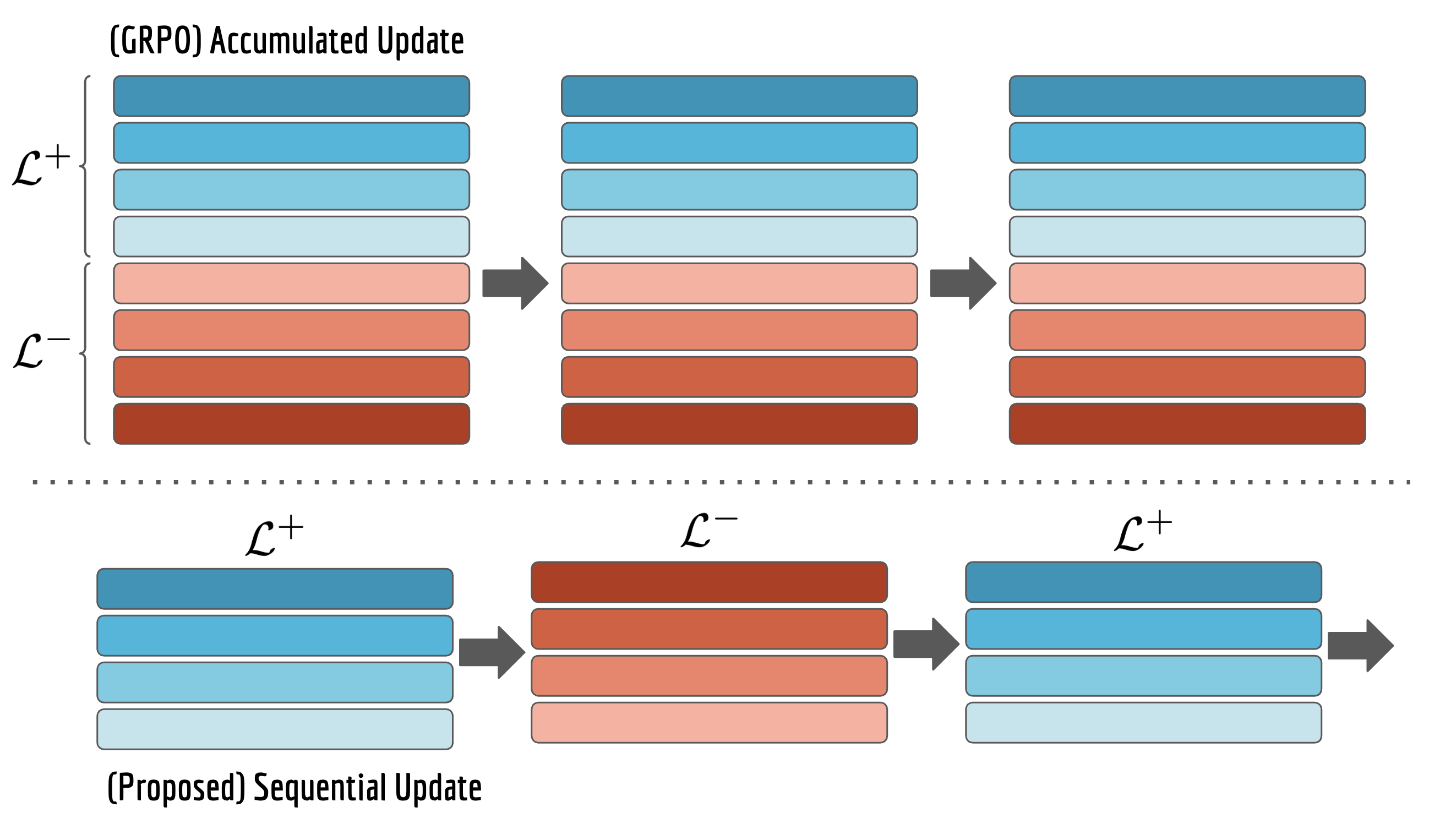
Setup: Seuential Updates between Loss Functions

In full-batch training, a gradient update step is given by: \[ \theta_{t+1} \leftarrow \theta - \frac{\eta}{B} \sum_{i=1}^B \nabla \mathcal{L}_i(\theta_t) \] Consider the following mini-batch training (we repeat the calculation in Section 2.2 of Smith et al.): \begin{aligned} \theta_1 &= \theta - \frac{\eta}{B} \nabla \mathcal{L}_1(\theta) \\ \theta_2 &= \theta - \frac{\eta}{B} \left( \nabla \mathcal{L}_1(\theta) + \nabla \mathcal{L}_2(\theta) \right) + \frac{\eta^2}{B^2} \nabla^2 \mathcal{L}_2(\theta) \mathcal{L}_1(\theta) + O((\eta / B)^3) \\ \vdots \\ \theta_m &= \underbrace{\theta - \frac{\eta}{B} \sum_{b = 1}^m \nabla \mathcal{L}_b(\theta)}_{\text{full batch update}} + \underbrace{\frac{\eta^2}{B^2} \sum_{b_1 = 1}^m \sum_{b_2 = 1}^{b_1 - 1} \nabla^2 \mathcal{L}_{b_1}(\theta) \nabla \mathcal{L}_{b_2}(\theta)}_{\text{correction term}} + O\left(m^3 \left(\frac{\eta}{B}\right)^3\right)\\ \end{aligned}

What if we introduce different loss functions at different mini-batch steps? Assume that we have two loss functions $\mathcal{L}^+$ and $\mathcal{L}^-$. For all even-indexed steps, we use $\mathcal{L}^+$. For all odd-indexed steps, we use $\mathcal{L}^-$. As a warm-up, let's assume no mini-batch noise. What does the correction term become? \begin{aligned} \sum_{b_1=1}^m\nabla^2 \mathcal{L}_{b_1}(\theta) \sum_{b_2=1}^{b_1-1} \nabla \mathcal{L}_{b_2}(\theta) = ( \frac{m^2}{2} - m ) \underbrace{\nabla^2 \mathcal{L}(\theta)\nabla \mathcal{L}(\theta)}_{ \mathcal{L} = \mathcal{L}^+ + \mathcal{L}^- } + \frac{m}{2} \nabla^2 \mathcal{L}^+(\theta) \nabla \mathcal{L}^-(\theta) + O(m^3 (\eta / B)^3) \end{aligned}

Set $m = B$ (one epoch consists of $B$ mini-batch steps). The correction term can be further simplified as: \[ \eta^2 \left[ \frac{B-2}{4B} \nabla \|\nabla \mathcal{L}\|^2 + \frac{1}{2B} \nabla^2 \mathcal{L}^+(\theta) \nabla \mathcal{L}^-(\theta) \right] \]

Implicit Bias of Gradient Accumulation

Now we relax the assumption that there are no mini-batch noise. Assume two sets of losses; at step $2k$, we sample from $\mathcal{L}^+_k$. At step $2k+1$, we sample from $\mathcal{L}^-_{k}$. To bring in some intuition, this corresponds to if we interleave GA on a randomly sampled batch of dispreferred outputs and GD on a randomly sampled batch of preferred outputs. If we further assume that each batch is computed on-policy, this would correspond to a sequential decomposition of RL algorithms like GRPO.

The original correction term (without coefficients) now becomes: \begin{aligned} \sum_{b_1=1}^m\nabla^2 \mathcal{L}_{b_1}(\theta) \sum_{b_2=1}^{b_1-1} \nabla \mathcal{L}_{b_2}(\theta) &= \sum_{k_1 = 1}^{B/2} \nabla^2 \mathcal{L}^-_{k_1} \sum_{k_2 = 1}^{k_1 - 1} \nabla \mathcal{L}^-_{k_2} + \sum_{k_1 = 1}^{B/2} \nabla^2 \mathcal{L}^-_{k_1} \sum_{k_2 = 1}^{k_1 - 1} \nabla \mathcal{L}^+_{k_2} \\ & \quad + \sum_{k_1 = 1}^{B/2} \nabla^2 \mathcal{L}^+_{k_1} \sum_{k_2 = 1}^{k_1} \nabla \mathcal{L}^-_{k_2} + \sum_{k_1 = 1}^{B/2} \nabla^2 \mathcal{L}^+_{k_1} \sum_{k_2 = 1}^{k_1 - 1} \nabla \mathcal{L}^+_{k_2} \end{aligned} We take the expecatation of the above correction term with respect to all permutations $\pi$ of pairs of $\mathcal{L}^+_{k_1}$ and $\mathcal{L}^-_{k_2}$. That is, adding $\mathbb{E}$ replaces indeces $k_i$ with $\pi(k_i)$, summing over all permutations $\pi$ of $1,\dots,B/2$, and dividing by $(B/2)!$. After some dirty algebra, we get: \begin{equation} \begin{aligned} \mathbb{E} \left[ \sum_{b_1=1}^m\nabla^2 \mathcal{L}_{b_1}(\theta) \sum_{b_2=1}^{b_1-1} \nabla \mathcal{L}_{b_2}(\theta) \right] &= \frac{B-2}{4B} \nabla \|\nabla (\mathbb{E} \mathcal{L}_i^- + \mathbb{E} \mathcal{L}_i^+)/2\|^2 \\ & \quad - \frac{1}{2B} \nabla \mathbb{E} \| \nabla \mathcal{L}_i - \nabla (\mathbb{E} \mathcal{L}_i^- + \mathbb{E} \mathcal{L}_i^+)/2\|^2 \\ & \quad + \frac{1}{2B} \mathbb{E} \left[ \nabla^2 \mathcal{L}_i^+(\theta) \nabla \mathcal{L}_i^-(\theta) \right] \end{aligned}\tag{1} \end{equation} Note that the last term is asymmetric. This is because we always choose to start with $\mathcal{L}^-$. Suppose we fix the "interleaving" schedule but allow randomness in whether we start with $\mathcal{L}^+$ or $\mathcal{L}^-$. Then a simple relabeling trick shows that the last term should become: \[ \boxed{\frac{1}{4B} \nabla \mathbb{E} \left[ \nabla \mathcal{L}_i^- \cdot \nabla \mathcal{L}_i^+ \right]} \]

Interpretation

If the number of batches $B$ is large, the correction terms in Eq. (1) is dominated by the first term and there's no difference between the one we would got if $\mathcal{L}^+$ is the same as $\mathcal{L}^-$.

But when we look at this in the context of RLHF algorithms, things get a little bit more interesting. What we are comparing is not a full-batch-per-epoch training versus mini-batch updates. We are comparing one RL gradient update versus its sequential decomposition into smaller gradient updates into GA and GD losses.

In this setup, $B$ is effectively how many trajectories are sampled per single gradient update in RLHF. In reasonable compute budget, $B$ doesn't get bigger than 32.

So, despite small, the effect of implicit anti-penalization of gradient alignment is noticeable. We want to understand how (lack of) this implicit bias affects RLHF algorithms.

A recent paper from Prof. Mengdi Wang's lab is very relevant to our finding. They argue that what's called "gradient entanglement"—the gradient of preferred outputs and dispreferred outputs are too big—leads to common pitfalls in RLHF training like catastrophic likelihood displacement.

This is exactly what our implicit bias term mitigates. In their definition of gradient entanglement, they consider that the preferred ($y^+$) vs. dispreferred outputs ($y^-$) gradients are too aligned. This is equivalent to saying $\nabla \mathcal{L}^+(y^+) \cdot \nabla \mathcal{L}^+(y^-)$ being too big (they evaluate gradients on the same loss). Our implicit bias term rewards $\nabla \mathcal{L}^+(y^+) \cdot \nabla \mathcal{L}^-(y^-)$, which is equivalent to penalizing $\nabla \mathcal{L}^+(y^+) \cdot \nabla \mathcal{L}^+(y^-)$ when $\mathcal{L}^+ = - \mathcal{L}^-$.

Experiments

I did some preliminary experiments to see how strong this implicit bias really is, and whether it leads to better training stability. I trained Llama3-8B-Instruct on the GSM8K dataset, using GPT-4o as a teacher model that produce preferred step-by-step solutions. Then I created synthetic dispreferred solutions by introducing errors in the step-by-step solutions.

There are two training procedures, both using the AdamW optimizer:

• Accumulated gradient updates: each gradient update samples $B/2$ solutions from the preferred loss and $B/2$ solutions from the dispreferred loss, and accumulates their gradients from GD and GA losses, respectively. Learning rate $\eta$.
• Sequential gradient updates: first sample $B/2$ solutions from the teacher dataset, perform one GD gradient update, then sample $B/2$ solutions from the dispreferred dataset, perform one GA gradient update. Following this work, the learning rate is $\eta' = 1/\sqrt{2} \eta$.

During training I tracked the eval loss and the scalar product between $\nabla \mathcal{L}^+(y^+)$ and $\nabla \mathcal{L}^-(y^-)$ for each training procedure.

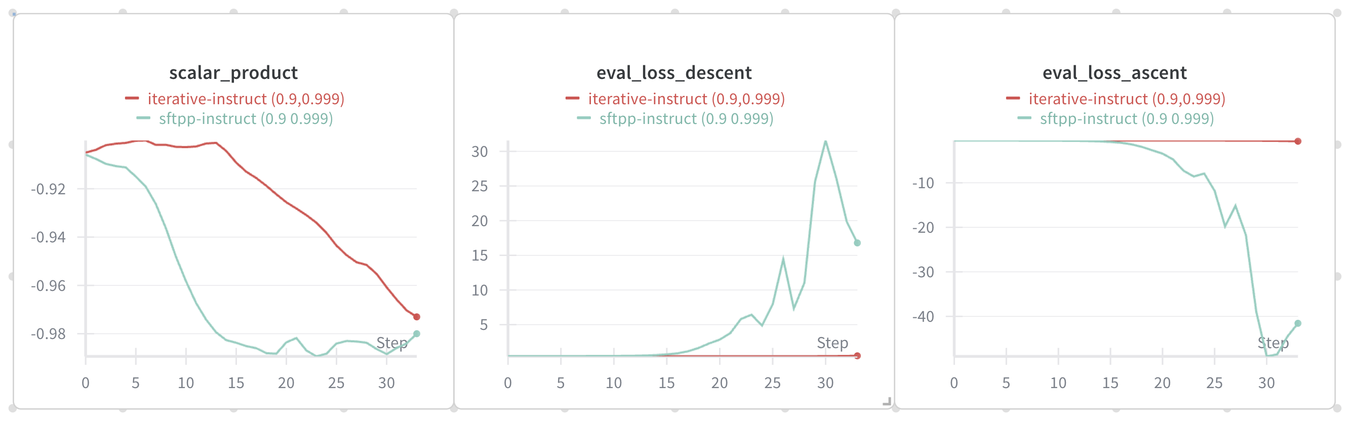
It is a surprising finding to me that this simple tweak can prevent catastrophic collapse already. As shown in the above result, SFTPP (green), which is the accumulated training setup, quickly diverges due to GA on stale dispreferred solutions from a teacher model. But by interleaving GD and GA updates, the divergence didn't happen! And as the first panel shows, we indeed observe the implicit bias at action: although both decreasing, the scalar product for the sequential update plan decreases slower.