
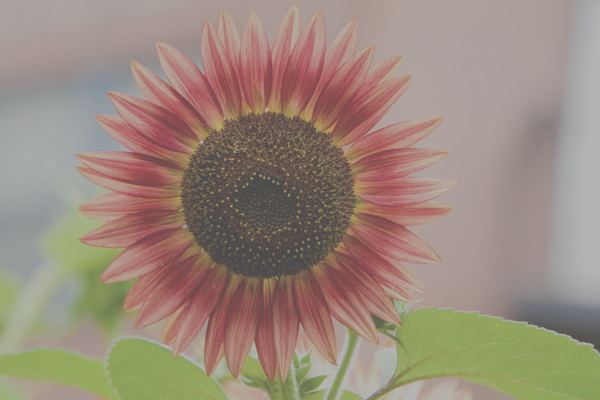
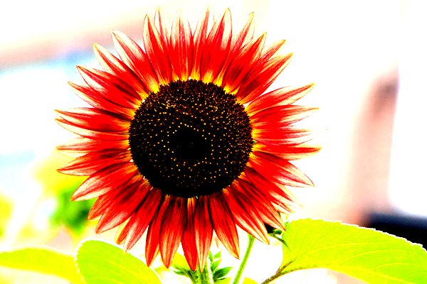
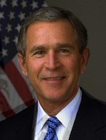
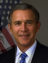
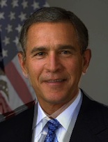
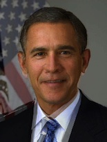
brightnessFilter( image, ratio )Changes the brightness of an image by blending the original colors with black/white color in a ratio. (When ratio>0, we blend with white to make it brighter; when ratio<0, we blend with black to make it darker.)
| -1 |
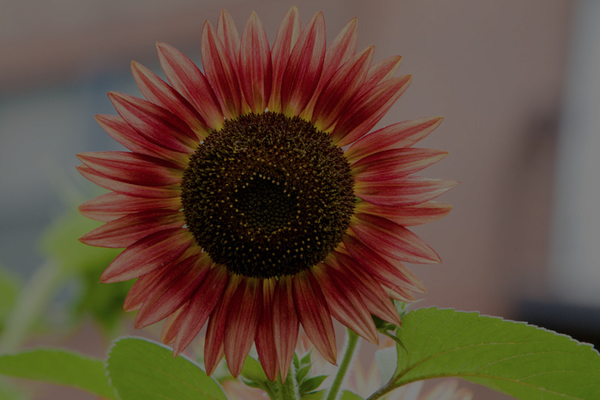 -0.5 |
 0 |
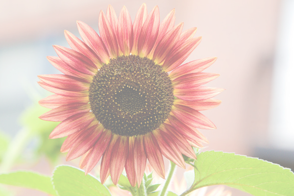 0.5 |
 1 |
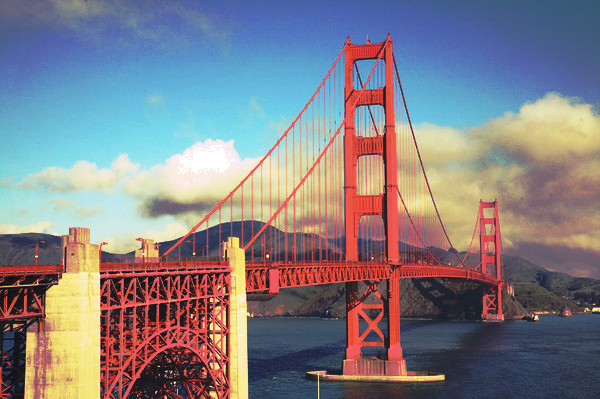
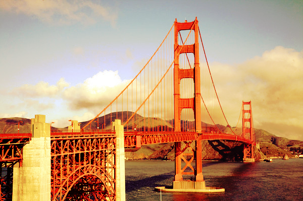
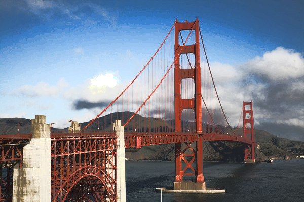
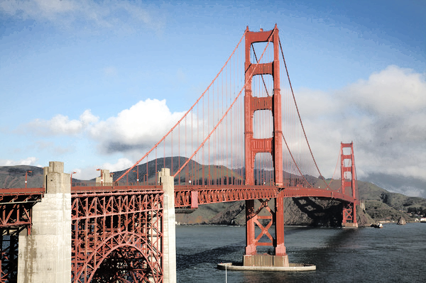
contrastFilter( image, ratio )Changes the contrast of an image by interpolating between a constant gray image (ratio=-1) with the average luminance and the original image (ratio=0). Interpolation reduces contrast, extrapolation boosts contrast, and negative factors generate inverted images. See Graphica Obscura and Wiki_Contrast (In Graphica Obscura' version, the slider is not uniformly ranged, so we remap the range [-1,1] to [0, infinite] using the following formula which is mentioned in Wiki_Contrast):
value = (value - 0.5) * (tan ((contrast + 1) * PI/4) ) + 0.5; -1 |
 -0.5 |
 0 |
 0.5 |
 1 |
gammaFilter( image, logOfGamma )Changes the image by applying gamma correction, V_out = Math.pow(V_in, \gamma), where \gamma = Math.exp(logOfGamma).
 -1 |
 -0.5 |
 0 |
 0.5 |
 1 |
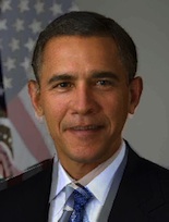
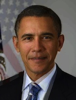
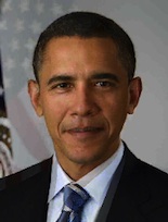
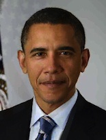
histeqFilter( image )Increase the contrast of the image by histogram equalization in HSL’s L channel, that is, remapping the pixel intensities so that the final histogram is flat. A low contrast image usually clumps most pixels into a few tight clusters of intensities. Histogram equalization redistributes the pixel intensities uniformly over the full range of intensities [0, 1], while maintaining the relationship between light and dark areas of the image.
Before |
After |
saturationFilter( image, ratio )Changes the saturation of an image by interpolating between a gray level version of the image (ratio=-1) and the original image (ratio=0). Interpolation decreases saturation, extrapolation increases it, and negative factors preserve luminance but invert the hue of the input image. See Graphica Obscura, its parameter
alpha=1+ratio in our slider.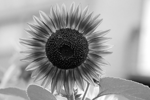 -1.0 |
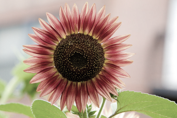 -0.5 |
 0 |
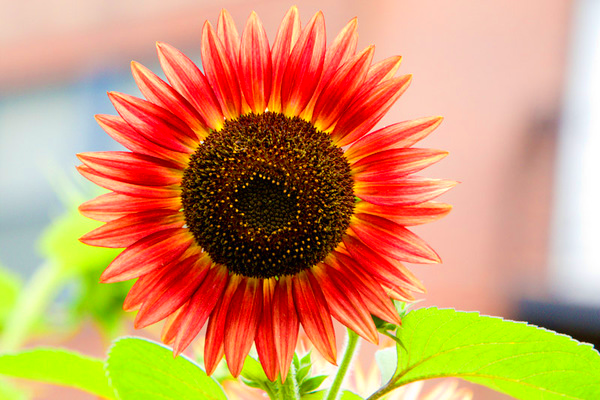 0.5 |
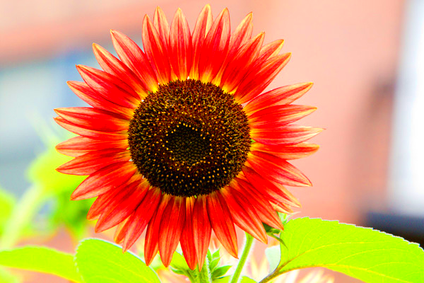 1 |
whiteBalanceFilter( image, hex )Adjust the white balance of the scene to compensate for lighting that is too warm, too cool, or tinted, to produce a neutral image. Use Von Kries method: convert the image from RGB to the LMS color space (there are several slightly different versions of this space, use any reasonable one, e.g. RLAB), divide by the LMS coordinates of the white point color (the estimated tint of the illumination), and convert back to RGB. (Image source)
Before correction: too warm |
After correction: neutral |
given white hex: #cee2f5 |
given white hex: #f5cece |
vignetteFilter( image, value )Darkens the corners of the image, as observed when using lenses with very wide apertures (ref). In the function, the value sets the innerRadius and outerRadius. It can be a value (which sets the innerRadius and makes outerRadius as default=1) or an array such as [0.1,0.7] or (0.1,0.7) which sets both the innerRadius and the outerRadius. The code for getting innerRadius and outerRadius from the value is already given. The image should be perfectly clear upto innerRadius, perfectly dark (black) at outerRadius and beyond, and smoothly increase darkness in the circular ring between. Both are specified as multiples of half the length of the image diagonal (so 1.0 is the distance from the image center to the corner).
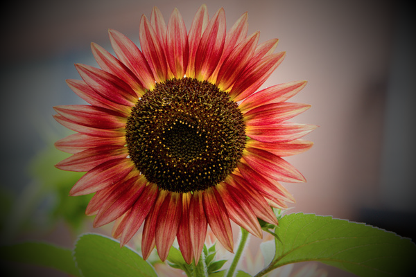
value=0.5, innerR:0.25, outerR:1 |
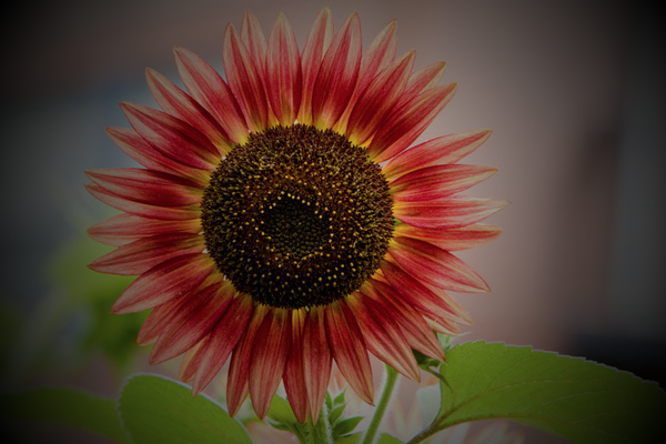
value=1, innerR:0.5, outerR:1 |
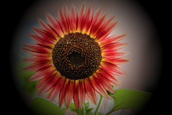
value=(0.5,0.5), innerR:0.25, outerR:0.75 |
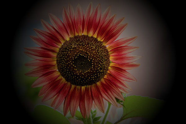
value=(1.0,0.5), innerR:0, outerR:0.75 |
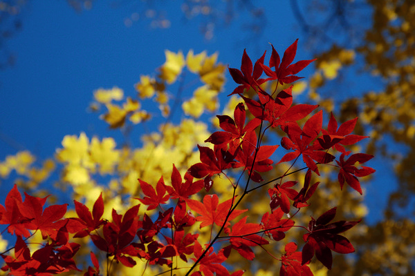
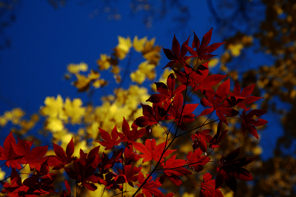
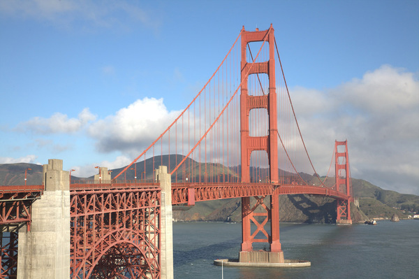
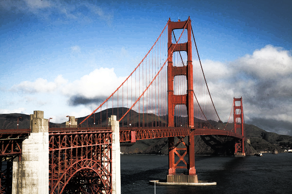
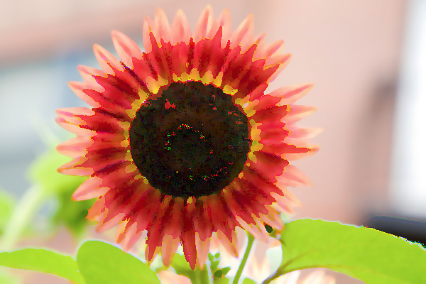
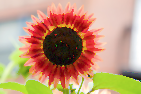
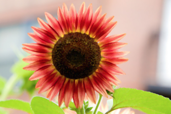
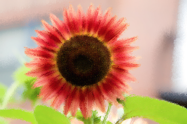
Filters.histMatchFilter = function( image, refImg, value )
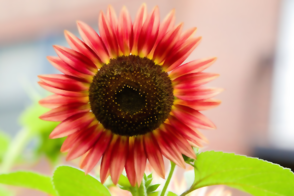
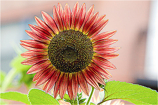
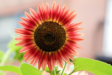
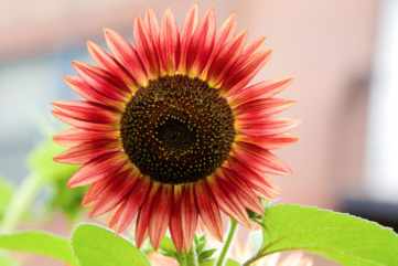
Adjusts the color/contrast of the input image by matching the histgram to refImg images. value can be used to control whether match the luminance or rgb channel.
The results in the first row below use the histogram matching in rgb channels, while the results in the second row matched only in luminance.
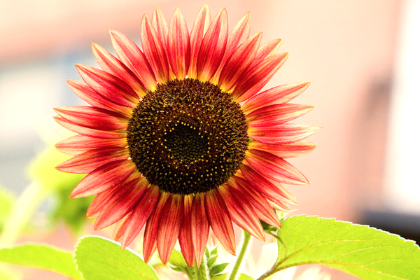
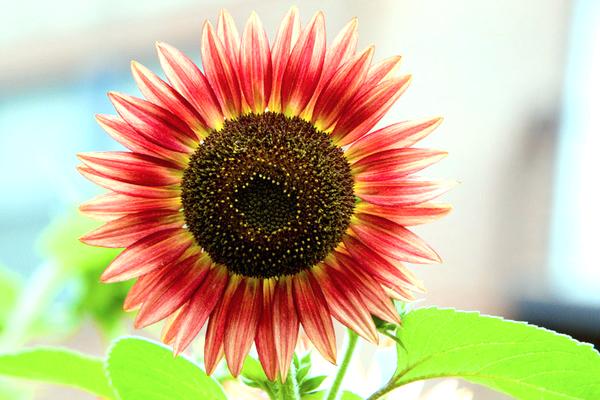
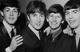
 reference image: town |
 reference image: flower |
 reference image: town |
 reference image: flower |
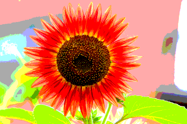
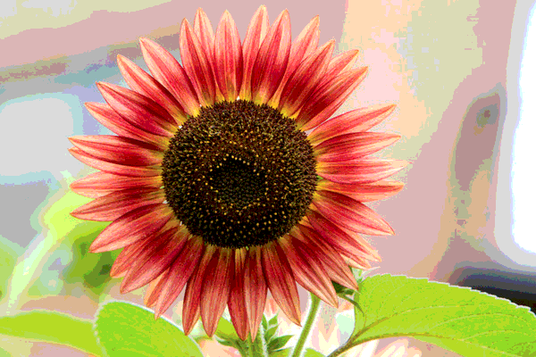
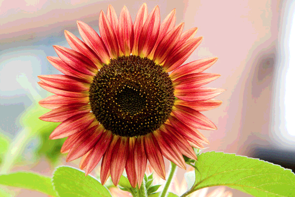
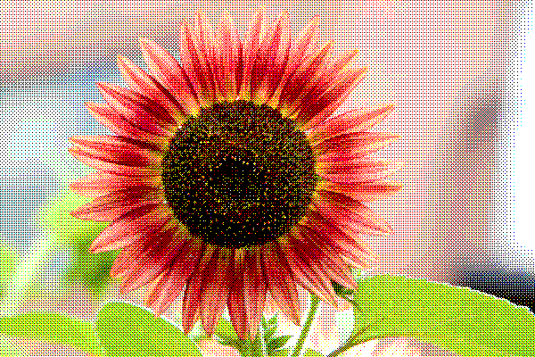
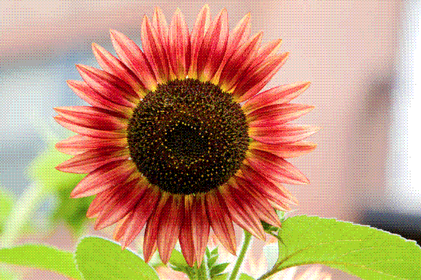
quantizeFilter( image, numBits )Converts an image to numBits bits per channel using uniform quantization.
The number of output levels per channel is numBits,
which are evenly distributed so that the lowest level is 0.0, the highest is
1.0. Every input value is to be mapped to the closest available output level.
 2 |
 4 |
 8 |
 16 |
 32 |
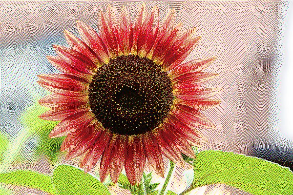
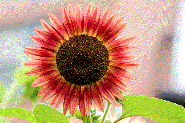
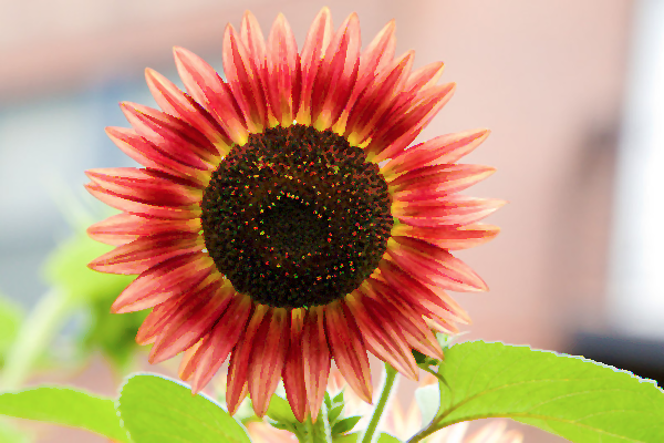
randomFilter( image, numBits )Converts an image to numBits bits per channel using random dithering. It is similar to uniform quantization, but random noise range in each unit is added to each component during quantization, so that the arithmetic mean of many output pixels with the same input level will be equal to this input level.
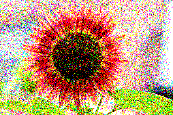 2 |
 4 |
 8 |
 16 |

32 |
orderedFilter( image, numBits )Converts an image to numBits bits per channel using ordered dithering. The following examples used the pattern
| Bayer4 | = | 15 | 7 | 13 | 5 |
| 3 | 11 | 1 | 9 | ||
| 12 | 4 | 14 | 6 | ||
| 0 | 8 | 2 | 10 |
 2 |
 4 |
 8 |
 16 |

32 |
floydFilter( image, numBits )Converts an image to numBits per channel using Floyd-Steinberg dither with error diffusion. Each pixel (x,y) is quantized, and the quantization error is computed. Then the error is diffused to the neighboring pixels (x + 1, y), (x - 1, y + 1), (x, y + 1), and (x + 1, y + 1) , with weights 7/16, 3/16, 5/16, and 1/16, respectively.
 2 |
 4 |
 8 |
 16 |
32 |
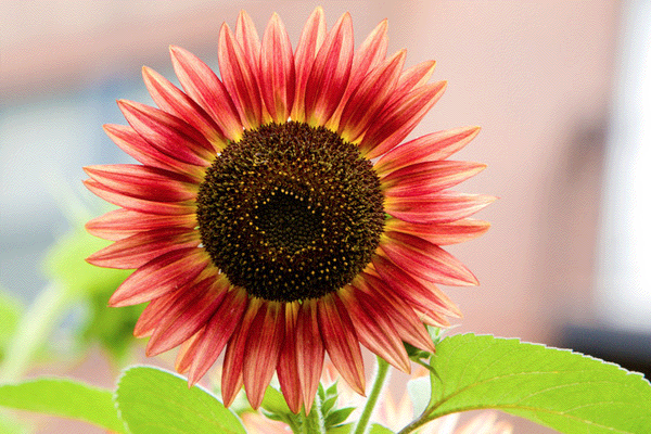
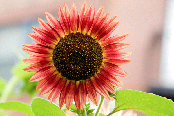
gaussianFilter( image, sigma )Blurs an image by convolving it with a Gaussian filter. In the examples below, the Gaussian function used was
Math.round(2*sigma)*2+1. 1 |
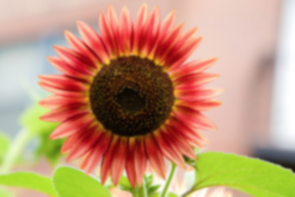 2 |
 3 |
 4 |
 5 |
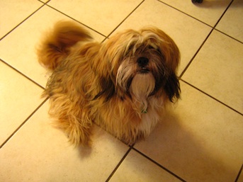
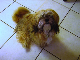
medianFilter( image, winR )Blurs an image by replacing each pixel by the median of its neighboring pixel((2*winR+1)x(2*winR+1)). So the results in the first row are done by doing median filter in RGB channel separately, the results in the second row are done by getting the median pixel sorted by their luminance values.
 1 |
 2 |
 3 |
 4 |
 5 |
 1 |
 2 |
 3 |
 4 |
 5 |
bilateralFilter( image, value ), where value = sigmaR(sigmaS=1 in this case) or [sigmaR, sigmaS]Blurs an image by replacing each pixel by a weighted average of nearby pixels. The weights depend not only on the euclidean distance of pixels but also on the pixel difference, for the pixel difference it could either be luminance difference or L2 distance in color space. Consider the pixel I(i,j) located in (i,j), the weight of pixel I(k,l) follows the following equation:

sigmaR by sqrt(2)*winR. If we don't take this factor into consideration, the result will be dominated by the spatial term, and will have similar results as gaussian blur.
You set the filter window size to 2* Math.round( max(sigmaR,sigmaS)*3 ) + 1. sigmaR=1 |
 sigmaR=2 |
 sigmaR=3, sigmaS=0.5 |
 sigmaR=4, sigmaS=2 |
 sigmaR=5, sigmaS=3 |
sharpenFilter( image )Sharpen edges in an image by convolving it with the edge kernel as belows and add it to the original image:
|
-1 |
-1 |
-1 |
|
-1 |
8 |
-1 |
|
-1 |
-1 |
-1 |
scaleFilter( image, ratio )Scales an image in width and height by ratio. The result depends on the current sampling method (point, bilinear, or Gaussian). In the example below, gamma=1, the window radius of the Gaussian filter is 3, ratio = 0.7.
 Point |
 Bilinear |
 Gaussian |
rotateFilter( image, ratio )Rotates an image by the given angle, in radians (a positive angle implies clockwise rotation) . The result depends on the current sampling method (point, bilinear, or Gaussian). In the example below, gamma=1, the window radius of the Gaussian filter is 3, ratio = 0.2.
 Point |
 Bilinear |
 Gaussian |
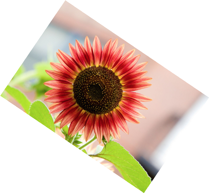
swirlFilter( image, ratio )Warps an image using a creative filter of your choice. In the following example, each pixel is mapped to its corresponding scaled polar coordinates, here ratio = 0.4.
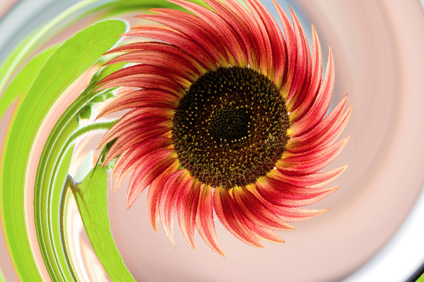 Point |
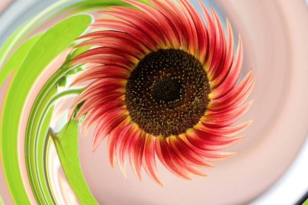 Bilinear |

Gaussian |
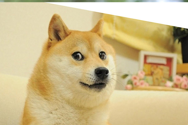
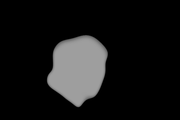
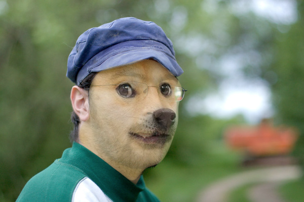
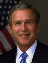
compositeFilterFile( backgroundImg, foregroundImg, alphaImg ) orComposites the foreground image over the background image, using the alpha file of the foreground image as a mask or using a alpha parameter to blend two images. You can use an image editor of your choice to generate the input images you need.
compositeFilter( backgroundImg, foregroundImg, alpha )
backgroundImg |
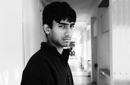
foregroundImg |
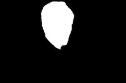
alphaImg |
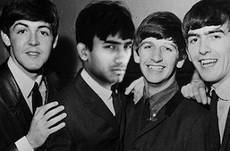
Result |
backgroundImg |
foregroundImg |
alphaImg |
Result |
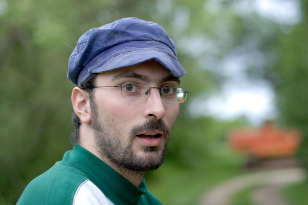
morphFilter( initialImg, finalImg, lines, alpha )Morph two images using [Beier92].
initialImg and finalImg are the before and after images, respectively. lines are corresponding line segments to be aligned.
alpha is the morph time: it can be a number between 0 and 1 indicating which point in the morph sequence should be returned, or can be (start:step:end) to define a morph sequence.

0 |
0.11 |
0.22 |
0.33 |
0.44 |
0.56 |
0.67 |
0.78 |
0.89 |
1 |
 |
alpha=(0:0.1:1) for
the example images and morph lines provided with the assignment zip,
together with a still frame at alpha=0.5: |
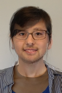 |
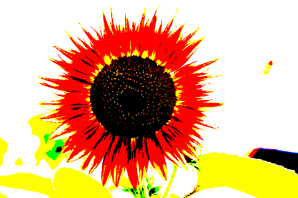
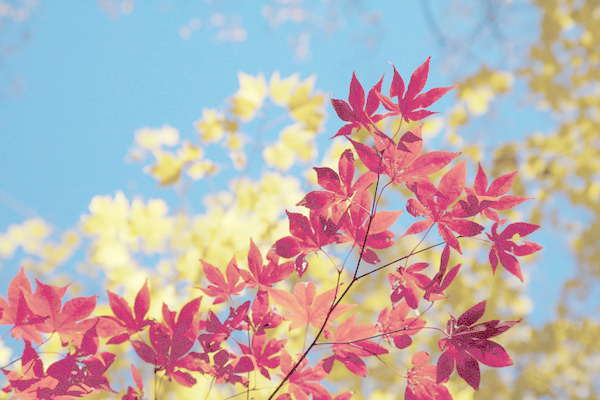
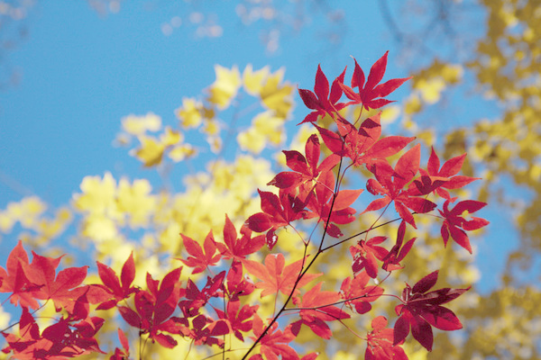
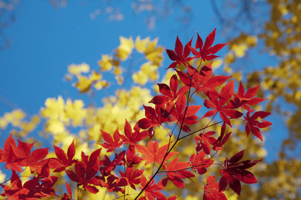
paletteFilter( image, colorNum )extracts colorNum colors as a palette to represent colors in the image. Here we use k-means method to extract color palette in the image with grid acceleration.
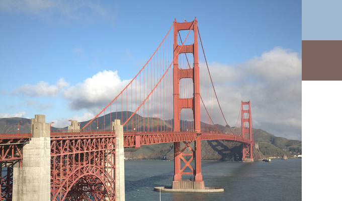 colorNum = 2 |
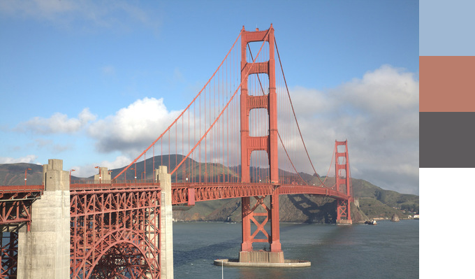 colorNum = 3 |
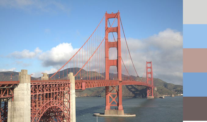 colorNum = 5 |