


COS 341, October 6, 1997Handout Number 7
Some Probability Theory
Let X be a random variable on a probability space
 . We define
 , and
Var(X)= E(Z), where
, and
Var(X)= E(Z), where 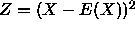 .
(Note that E(X) is a real number t, and
for all
.
(Note that E(X) is a real number t, and
for all  , the random
variable X-E(X) has value X(u)-t,
the random variable Z has value
, the random
variable X-E(X) has value X(u)-t,
the random variable Z has value 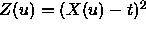 . Clearly
  .)
The standard deviation
.)
The standard deviation  is
defined to be
is
defined to be  .
Intuitively, the value E(X) tells you what the average value
of X you can expect, if you perform many many
experiments; the variance
gives you some idea on how close to E(X) you
expect to see the typical value of X fall in these experiments.
This last statement is made more precise in the
Chebyshev's Inequality below.
.
Intuitively, the value E(X) tells you what the average value
of X you can expect, if you perform many many
experiments; the variance
gives you some idea on how close to E(X) you
expect to see the typical value of X fall in these experiments.
This last statement is made more precise in the
Chebyshev's Inequality below.
Recall that, if 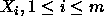 are random variables
in
are random variables
in  and
and  are real numbers, then the
random variable
are real numbers, then the
random variable  is
defined by
is
defined by  .
The following important formula was derived in class.
.
The following important formula was derived in class.
Linearity of Expected Value

As an example to illustrate all these discussions,
let , where  and
p(a)=0.2, p(b)=0.13, p(c)=0.17, p(d)=0.1,
p(e)=0.1, p(f)=0.2, p(g)=0.04, p(h)=0.06.
Let X be the random variable on
with X(a)=1, X(b)=X(c)=3, X(d)=X(e)=X(f)=4, X(g)
=X(h)=9. Then by defintion
and
p(a)=0.2, p(b)=0.13, p(c)=0.17, p(d)=0.1,
p(e)=0.1, p(f)=0.2, p(g)=0.04, p(h)=0.06.
Let X be the random variable on
with X(a)=1, X(b)=X(c)=3, X(d)=X(e)=X(f)=4, X(g)
=X(h)=9. Then by defintion

Let t=E(X) denote the above value. Then by definition

The numerical values of E(X) and Var(X) can be calculated straightforwardly from these formulae. We shall not do the calculation here. Rather, we calculate them in a slightly different way.
Clearly,  ,
,  ,
,
 , and
, and  .
.
Now, by definition, .
When X takes on only nonnegative integer values, we
can rewrite it as

Similarly, from the definition of Var(X), we can derive

Thus, for the example above,

and

Also we have  .
.
The following inequality
says that, taking an experiment according to , the
probability of seeing the value of X deviating from E(X) by
c (or more) standard deviations is less than  .
.
Chebyshev's Inequality Let c>0,

Proof If Var(X)=0, then
X(u)=E(X) for all (why?), and
the Inequality is clearly true.
Assume Var(X)>0. Let Y=X-E(X). Then
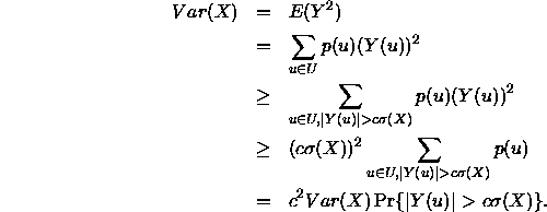
This implies the Inequality. 
For example, take c=10. The probability for X to deviate from
E(X) by  (or more) is less than 1 percent.
Another useful formula

Proof Let t=E(X) and  . Note that
 for all .
Thus
for all .
Thus  expresses the random
variable Z as a linear combination of the
random variables
expresses the random
variable Z as a linear combination of the
random variables  . By the linearity of
the expected value, we have
. By the linearity of
the expected value, we have  ,
which proves (3).
,
which proves (3).
Generating Functions
We have seen earlier that generating functions are useful for
evaluating sums such as 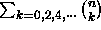 .
We now demonstrate that the generating functions
are also useful for evaluating E(X) and
Var(X), when X take on only nonnegative integer values.
Take any such X, let
.
We now demonstrate that the generating functions
are also useful for evaluating E(X) and
Var(X), when X take on only nonnegative integer values.
Take any such X, let 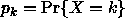 . Define

Then

and

Thus,

and

It follows that

And
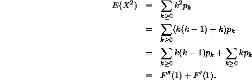
By (3) this gives

As an application, consider the example of tossing a fair
coins n times, and let X be the number of Heads in
the sequence. Then  and
and
 . Clearly,
 and
and
 .
Thus F'(1)=n/2 and
.
Thus F'(1)=n/2 and  .
From (5) we have
.
From (5) we have  .
.