
This lab is meant to show you how Python programming might be useful in the humanities and social sciences. As always, this is a very small taste, not the whole story, but if you dig in, you'll learn a lot, and you might well get to the point where you can write useful programs of your own.
This lab is newish, so there are sure to be murky bits and rough edges. Don't worry about details, since the goal is for you to learn things, but let us know if something is confused or confusing.
Please read these instructions all the way through before beginning the lab.
Do your programming in small steps, and make sure that each step works before moving on to the next. Pay attention to error messages from the Python compiler; they may be cryptic and unfamiliar, but they do point to something that's wrong. Searching for error messages online may also help explain the problem.
Most Python programming uses libraries of code that others have written, for an enormous range of application areas. This lab is based on two widely used libraries: the Natural Language Toolkit (NLTK), which is great for processing text in English (and other languages), and Matplotlib, which provides lots of ways to plot your data.
NLTK is documented in an excellent free online book called Natural Language Processing with Python, by Steven Bird, Ewan Klein, and Edward Loper. The book alternates between explanations of basic Python and illustrations of how to use it to analyze text. We will use only a handful of NLTK's features, primarily ones found in the first chapter, but you should skim the first three or four chapters to get a sense of what NLTK can do for you.
You are welcome to use other libraries as well. This lab is meant to encourage you to experiment; we're much more interested in having you learn something than forcing you through a specific sequence of steps.
Normally you would run Python on your own computer, but for this lab you should use Google Colab, which provides an interactive web-based environment for developing and running Python code. You don't have to worry about text editors, command lines, or local files, nor about losing your work if something crashes. When Python runs within the confines of a browser, there are some limitations on what you can do --- for example, it may not be possible to read information from the file system on your computer or to store information there --- but you can usually access anything on the Internet.
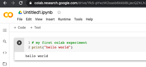
To get started, go to the Colab web site, select File, then New notebook, then type your program in the "+ Code" box; you can use a "+ Text" box to add explanatory comments, though for this lab, it's probably easier to just put comments in the code. Here's the first example:
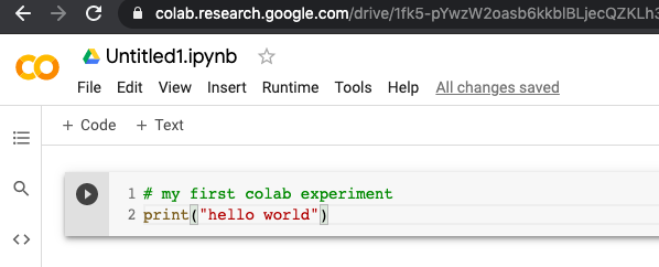
Clicking the triangle icon will compile and run the program, producing this:
You can add as much code as you like; just add more sections as you evolve a system.
Colab provides a very useful service: as you type, or if you hover over something, it will give you information about how to use a statement or possible continuations of what you are typing, like this:

Let's download a book from the Internet and do some experiments. I've chosen Pride and Prejudice from Project Gutenberg, but you can use anything else that you like. It can be a help if you're familiar with whatever document you choose so you can think of questions to explore and spot places where something doesn't look right, though you might also decide to look at material that isn't too familiar.
In this part, please follow along with Austen or a book of your own. Later on you will get to do further explorations with your chosen text. You might find that some of the outputs differ from what is shown here; it seems that even the sacred Austen text is subject to updates over time.
In the rest of the lab,
we will use pink blocks like this for code
and green blocks like this for output produced by that code.It is strongly recommended that you start a new Code block for each of the pink blocks; that will help you keep track of where you are, and it's more efficient than repeatedly downloading the original text.
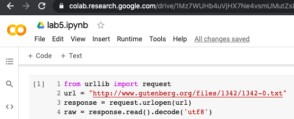
This sequence of Python statements fetches the whole text, including boilerplate at the beginning and end:
from urllib import request
url = "http://www.gutenberg.org/files/1342/1342-0.txt"
response = request.urlopen(url)
raw = response.read().decode('utf8')  # reads all the bytes of the file
                                      # in utf-8 format, a form of Unicode
In Colab, this would look like this before it has been run.
After it has been run, the variable raw contains a long string of Unicode characters. We can compute how long the text is, and we can print some or all of it:
print(len(raw))
print(raw[1980:2420])
789417

      It is a truth universally acknowledged, that a single man in
      possession of a good fortune, must be in want of a wife.

      However little known the feelings or views of such a man may be
      on his first entering a neighbourhood, this truth is so well
      fixed in the minds of the surrounding families, that he is
      considered the rightful property of some one or other of their
      daughters.
The expression raw[start:end] is called a slice; it's a convenient feature of many programming languages. It produces the characters from position start to position end-1 inclusive, so in the case above, it provides the characters in positions 2240 to 2669. If you omit start, the slice starts at the beginning (character 0), and if you omit end, the slice ends at the last character (one position before end). Negative numbers count backwards from the end, so [-1000:] is the last thousand characters. You can experiment with statements like
print(raw[0:75])
print(raw[-1000:])
to figure out where the book text begins and ends. (Remember binary search?)
The start and end positions for this specific book were determined by experiment, which is not very general, though it's helpful for getting started. If you know what you're looking for, it's more effective to use the find function to locate the first occurrence of some text:
start = raw.find("It is a truth")
end = raw.find("wife.")       # Think about which wife you get
print(raw[start:end+5])       # Think about why +5
It is a truth universally acknowledged, that a single man in
      possession of a good fortune, must be in want of a wife.
Use your own numbers and text to find the beginning and end of the real text in your chosen book. Gutenberg books have a lot of boilerplate; the extra material at the end appears to be consistently marked with
*** END OF THE PROJECT GUTENBERG EBOOKAgain, we could find the end by experiment, but it's easier to let Python do the work:
end = raw.find("*** END OF THE PROJECT GUTENBERG EBOOK")
print(raw[end-140:end])
the warmest gratitude towards the persons
      who, by bringing her into Derbyshire, had been the means of
      uniting them.
Combining all this, we can define a new variable body that
contains exactly the text of the book:
start = raw.find("It is a truth")
end = raw.find("*** END OF THE PROJECT")
body = raw[start:end]
body = body.strip()  # remove spaces at both ends
len(body)
print(body[:80], "[...]", body[-80:])
768656
It is a truth universally acknowledged, that a single man in
      possession o [...] who, by bringing her into Derbyshire, had been the means of
      uniting them.
You can get an approximate word count by using Python's split function to split the text into an array of "words," which are the alphanumeric parts of the text that were separated by blanks or newlines. The result is an array of words, indexed from 0. The len function returns the number of items in the array, and again you can use the slice notation to see parts of the array.
words = body.split()  # creates a list "words" by splitting on spaces and newlines
print(len(words))     # len(list) is the number of items in the list
print(words[0:10])
121559
['It', 'is', 'a', 'truth', 'universally', 'acknowledged,', 'that', 'a', 'single', 'man']
Chapter 1 of the NLTK book uses a database of text materials that its authors have collected, and a variety of interesting functions that we won't try. You can certainly explore that, but here we are going to use our own data, which is a bit simpler and less magical, and requires only a small subset of what NLTK offers.
Before you can use functions from the NLTK package, you have to import it like this:
import nltk
words = nltk.tokenize.wordpunct_tokenize(body)  # produces a list, like split()
print(len(words))
print(words[0:10])
144001
['It', 'is', 'a', 'truth', 'universally', 'acknowledged', ',', 'that', 'a', 'single']
Notice that the number of "words" is quite a bit larger than the value computed by a simple split, and the words are subtly different as well: look at the word acknowledged and you'll see that the comma in the first occurrence is now a separate item. Separating punctuation in this way might well explain the difference in counts.
Of course, a comma is not a word, but that's a problem for another day.
Now let's look at vocabulary, which is the set of unique words. This doesn't really need NLTK; we can use functions that are part the standard Python library. The function set collects the unique items, and the function sorted sorts them into alphabetic order.
uniquewords = set(words)   # the set function collects one instance of each unique word
print(len(uniquewords))
sortedwords = sorted(uniquewords)  # sort the words alphabetically
print(sortedwords[:20])
6893
['!', '!)', '!—', '!”', '!”—', '&', '(', ')', '),', ').', ',', ',—', ',’', ',’—', ',”', ',”—',
It's clear that the punctuation is throwing us off the track,
so let's write code to discard it. We'll use a for
loop here, though Pythonistas would use the more compact but
less perspicuous code that has been commented out.
# realwords = [w.lower() for w in words if w[0].isalpha()]

realwords = []      # create an empty list (no elements)
for w in words:     # for each item in "words", set the variable w to it
  if w.isalpha():                 # if the word w is alphabetic
    realwords.append(w.lower())   # append its lowercase value to the list

rw = sorted(set(realwords))
print(len(rw))
print(rw[:10])
The result is a lot more useful, and the number of real words is
smaller now that the punctuation has been removed:
6248
['a', 'abatement', 'abhorrence', 'abhorrent', 'abide', 'abiding', 'abilities', 'able', 'ablution', 'abode']
We can look at other parts of the list of words, such as the last ten words:
print(rw[-10:])
['younge', 'younger', 'youngest', 'your', 'yours', 'yourself', 'yourselves', 'youth', 'youths', 'à']and, with a loop, some excerpts from the list:
for i in range(0,len(rw),1000):  # range produces a list of indices from 0 to len in steps of 1000
  print(rw[i:i+10])              # for each index, print a slice that starts there
['a', 'abatement', 'abhorrence', 'abhorrent', 'abide', 'abiding', 'abilities', 'able', 'ablution', 'abode']
['command', 'commanded', 'commencement', 'commendable', 'commendation', 'commendations', 'commended', 'commerce', 'commiseration', 'commission']
['establishment', 'estate', 'estates', 'esteem', 'esteemed', 'estimable', 'estimated', 'estimation', 'etc', 'etiquette']
['injured', 'injuries', 'injuring', 'injurious', 'injury', 'injustice', 'inmate', 'inmates', 'inn', 'innocence']
['patronage', 'patroness', 'pause', 'paused', 'pauses', 'pausing', 'pavement', 'pay', 'paying', 'payment']
['service', 'serviceable', 'services', 'servility', 'serving', 'set', 'setting', 'settle', 'settled', 'settlement']
['visited', 'visiting', 'visitor', 'visitors', 'visits', 'vivacity', 'vogue', 'voice', 'void', 'volatility']
nltk.download('stopwords')  # has to be done once
text = nltk.Text(words)
text.collocations()
Lady Catherine; Miss Bingley; Sir William; Miss Bennet; Colonel
Fitzwilliam; dare say; Colonel Forster; young man; thousand pounds;
great deal; young ladies; Miss Darcy; Miss Lucas; went away; next
morning; said Elizabeth; young lady; depend upon; Lady Lucas; soon
afterwards
If we had not used stopwords, there would be more uninteresting collocations like of the or and she.
text.concordance("Darcy")
Displaying 25 of 417 matches:
 the gentleman ; but his friend Mr . Darcy soon drew the attention of the room
st between him and his friend ! Mr . Darcy danced only once with Mrs . Hurst an
 and during part of that time , Mr . Darcy had been standing near enough for he
ess his friend to join it . “ Come , Darcy ,” said he , “ I must have you dance
ndsome girl in the room ,” said Mr . Darcy , looking at the eldest Miss Bennet
. Bingley followed his advice . Mr . Darcy walked off ; and Elizabeth remained
tion , the shocking rudeness of Mr . Darcy . “ But I can assure you ,” she adde
ook it immediately . Between him and Darcy there was a very steady friendship ,
...
text.dispersion_plot(["Elizabeth", "Jane", "Lydia", "Kitty", "Mary"])
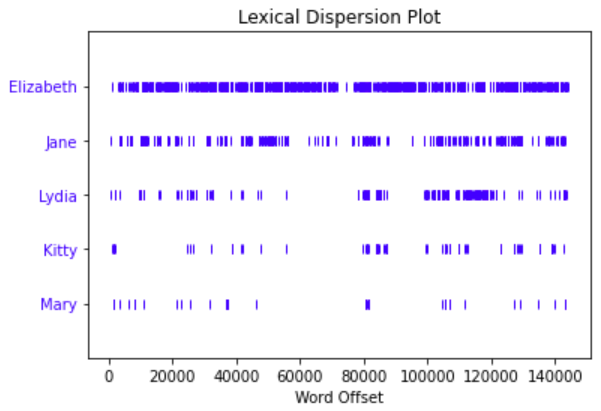
It's clear that Elizabeth is the main character, and Mary is sort of a bit player. (For a bit of alternate history, check out The Other Bennet Sister, by Janice Hadlow, available in Firestone.)
import matplotlib
fd = nltk.FreqDist(realwords)  # fd is a variable that has multiple components
print(fd.most_common(20))      # including some functions!
fd.plot(20)
[('the', 4333), ('to', 4163), ('of', 3611), ('and', 3585), ('her', 2202), ('i', 2048), ('a', 1948), ('in', 1879), ('was', 1844), ('she', 1691), ('that', 1540), ('it', 1535), ('not', 1421), ('you', 1326), ('he', 1325), ('his', 1257), ('be', 1239), ('as', 1182), ('had', 1172), ('for', 1058)]
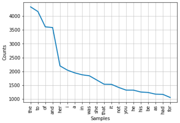
The numbers indicate the number of times each word occurs in the document; as might be expected, "the" is most common. We can also see how often the names of our hero and heroine appear:
print(fd['elizabeth'], fd['darcy'])
634 417
Your assignment is do experiments like what we did above, but for some text that appeals to you (except don't use Pride and Prejudice. You don't have to follow this in detail; the goal of this lab is for you to learn a bit of Python, see how it can be used for text analysis, and have some fun along the way.
What else can you do that isn't listed here? You might look at the NLTK book again for inspiration. Chapter 1 includes several ideas that we did not look at above, including the functions similar and common_contexts in section 1.3 to list words that appear in similar contexts, and a computation of unusually long words in section 3.2. There are also more frequency distribution functions in section 3.4.
Save your Colab notebook in a file called lab6.ipynb, using File / Download .ipynb. The .ipynb file should not be too large, say no more than a megabyte. To save space, delete the outputs of the various code sections before you download, since they can be recreated by re-running your code. We will experiment with your experiments by running your notebook, so please make sure it works smoothly for us. Get a friend to run through yours to see if it works for him or her.
Upload lab6.ipynb to the CS tigerfile for Lab 6 at https://tigerfile.cs.princeton.edu/COS109_F2022/Lab6.