COS 429 - Computer Vision

Fall 2019

Assignment 4: Deep Learning

Part II. Adding a hidden layer

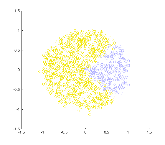
The "network" that you trained in part 1 was rather simple, and still only supported a linear decision boundary. The next step up in complexity is to add additional nodes to the network, so that the decision boundary can be made nonlinear. That will allow classifying datasets such as this one:

We will implement a simple network with only "fully connected" layers, "relu", and the logistic function – Here is a simple example of the architecture that we will use. It contains one "hidden" fully connected layer with two neurons (u and v) and one output layer with one neuron:

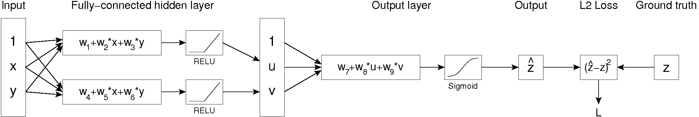
For convenience, we've given the names $u$ and $v$ to the neurons of the two hidden nodes, and $\hat{z}$ to the final output after it has been squished by the logistic function. As before, $z$ is the ground-truth label. The different $w$ are the weights to be learned during training, then used during testing.

To train this network using SGD, we need to evaluate $$ \nabla L = \begin{pmatrix} \frac{\partial L}{\partial w_1} \\ \frac{\partial L}{\partial w_2} \\ \frac{\partial L}{\partial w_3} \\ \vdots \end{pmatrix} $$

As discussed in class, evaluating these partial derivatives is done using "backpropagation", which is just a fancy name for repeatedly applying the chain rule of differentiation, collapsing into a row vector for efficiency, and repeating. For example, suppose we wish to evaluate $\frac{\partial L}{\partial w_5}$. Tracing back through the network to find the dependency, we know that $L$ depends on $\hat{z}$, which depends on $v$, which in turn depends on $w_5$. So, using the chain rule, we can write $$ \frac{\partial L}{\partial w_5} = \frac{\partial L}{\partial \hat{z}} \frac{\partial \hat{z}}{\partial v} \frac{\partial v}{\partial w_5} $$ and then proceed to write out all of those partial derivatives: $$ \frac{\partial L}{\partial w_5} = \bigl( 2 \; (\hat{z} - z) \bigr) \bigl( \hat{z} \; (1 - \hat{z}) \; w_9 \bigr) \bigl( Z(v) \; x \bigr) $$ Here $Z$ is a function that returns 1 if its argument is $>$ 0 and 0 otherwise. (Note that it's critical for this to be defined as $>$ 0 and not $\geq$ 0.) $Z$ is the derivative of RELU, just as $\hat{z}\;(1-\hat{z})$ is the derivative of the sigmoid.

In practical implementations, for efficiency and modularity, each layer of the network supports a backwards layer which takes as inputs the derivatives of the loss with respect to the outputs of the layer, and returns the derivatives with respect to the inputs of the layer (inputs includes the input vector 'x' to the layer, as well as the parameters at that layer). In order to get comfortable with backprop, we suggest that you write out the partial derivatives of $L$ at each layer before moving forward.

The starter code for this part defines a function tinynet_sgd that supports the above architecture, but with a few important generalizations:

• The input vector can be of arbitrary dimensionality (not just two scalars 'x' and 'y'). It is a row vector in the code to be consistent with standard matrix calculus conventions.
• Rather than passing ones around, a separate bias vector 'b' is stored at each fully connected layer. Each fully connected layer is then defined as x*W + b, where x is a (row vector) input. This simplifies the derivatives you will have to compute.
• There can be an arbitrary number of chained fully-connected hidden layers before the output layer (chaining them together is handled for you), and they can each have an arbitrary number of neurons. The network architecture is specified as a vector 'layers', which for the diagram above would be '[2]' (e.g. one hidden layer with two neurons, 'u' and 'v'. The output layer is implicit). For a network with two hidden layers, the first with three neurons and the second with two neurons, 'layers' would be '[3,2]'.

Do the following:

• Download the starter code for this part.
• Read through the codebase, starting with test_tinynet.py and tinynet_sgd.py. They contain the main entrypoints to this part of the assignment. There are many hints and clarifications throughout the code comments, so please read all code in this folder.
• Implement logistic.py, relu.py, and fully_connected.py. These are the forward layers of the network.
• Implement logistic_backprop.py, relu_backprop.py, and fully_connected_backprop.py. These are the backwards layers of the network. Because fully_connected_backprop.py is the trickiest part of the assignment, but later code depends on it, we have provided fully_connected_backprop_gt.pyc. This is a compiled file that contains a correct implementation of fully_connected_backprop.py that you can call the same function fully_connected_backprop() after from fully_connected_backprop_gt import fully_connected_backprop. Feel free to write unit tests against this code, or to use it in place of fully_connected_backprop.py if (and only if) you get stuck. This file is just meant to act as a timesaver, as there is an always-available and standard way of writing unit tests for backprop code: using a finite difference approximation to estimate the gradients from the forward pass. You are on the honor code not to try to decrypt the .pyc, and to use your version of the function for the remaining parts of the assignment if you want full credit.
• Implement the body of tinynet_predict.py.
• Implement the backpropogation pass of the network in tinynet_sgd.py.
• Train the default network using SGD by running test_tinynet.py. Run it several times - you should see the network converging to different results. It should converge to a good result some, but not all, of the time.
• Experiment with different network architectures to get improved convergence and performance. Do additional layers always help? What about more neurons in each layer? How does the number of epochs and learning rate affect the network? Try a network with a constant number of neurons (i.e. 6,6,6) versus one with an hourglass shape (i.e. 9,6,3). Does one exhibit better accuracy or convergence properties than the other?

• In Assignment 4 code: all files from the starter code with your well commented implementations inside a folder called q2.
• In Assignment 4 written: a section in the README.pdf containing your short answer responses to the final bullet point's questions and your modified code snippets (Pleaes refer to the main page for Assignment 4).

• On to Part III
• Back to the main page for Assignment 4