COS 429 - Computer Vision

Fall 2019

Assignment 1: Image processing and feature detection

• 9/18/19: Clarified 4a) Hint #1: Make sure that the input image im to filteredGradient and cannyEdgeDetection are already greyscale and floats between 0 and 1 when passing them in.
• 9/18/19: Added in submission details and expected deliverables. Submission link will be available on Monday 9/23.
• 9/19/19: Updated hints for 4a). Don't worry about normalizing filters to sum up to 1.
• 9/20/19: Converted directions for nonmaximum suppression to radians for consistency.
• 9/23/19: Clarified the output format for HysteresisThresholding. It should be an np.float matrix with values of either 0 or 1, where 1 denotes edge pixel.

1. Pinhole camera model (5 pts)

Consider a pinhole camera with focal length $f$. Let this pinhole camera face a whiteboard, in parallel, at a distance $L$ between the whiteboard and the pinhole. Imagine a square of area $S$ drawn on the whiteboard. What is the area of the square in the image? Justify your answer.

2. Linear filters (20 pts)

You are expected to do this question by hand. Show all steps for full credit.

In class we introduced 2D discrete space convolution. Consider an input image $I[i,j]$ with an $m \times n$ filter $F[i,j]$. The 2D convolution $I * F$ is defined as: \[ (I*F)[i,j] = \sum_{k,l}I[i-k,j-l]F[k,l] \] Note that the above operation is run for each pixel \((i,j)\) of the result.

1. Convolve the 2x3 matrix \(I = [-1, 0, 2; 1, -2, 1] \) with the 3x3 matrix \(F = [-1, -1, -1; 1, 1, 1; 0, 0, 0] \). Use zero-padding when necessary. The output shape should be 'same' (same as the 2x3 matrix \(I\)).
   
   
2. Note that \(F\) is separable, i.e., it can be written as a product of two 1D filters: \(F_1 = [-1; 1; 0]\) and \(F_2 = [1, 1, 1]\). Compute \((I*F_1)\) and \((I * F_1) * F_2\), i.e., first perform 1D convolution on each column, followed by another 1D convolution on each row.
   
   
3. Prove that for any separable filter \(F = F_1F_2\): \[I*F = (I*F_1)*F_2\] Hint: expand the 2D convolution equation directly.

3. Difference-of-Gaussian (DoG) detector (25 pts)

1. Recall that a 1D Gaussian is: \[g_{\sigma}(x) = \frac{1}{\sqrt{2\pi}\sigma}\exp \left (-\frac{x^2}{2\sigma^2} \right ) \] Calculate the 2nd derivative of the 1D Gaussian with respect to \(x\) and plot it in Python (use \(\sigma=1\)). Submit all steps of your derivation and the generated plot in the PDF file you turn in.
   Hint: Create a large number of \(x\) using np.linspace, and get function outputs from those. You can then use Matplotlib to plot the function. If you are unfamiliar with Matplotlib, get started here.
   
   
2. Use Python to plot the difference of Gaussians in 1D given by \[D(x,\sigma,k) = \frac{g_{k\sigma}(x)-g_{\sigma}(x)}{k\sigma-\sigma}\] using k = 1.2, 1.4, 1.6, 1.8, 2.0. State which value of \(k\) gives the best approximation to the 2nd derivative with respect to \(x\). Assume \(\sigma=1\). You will need to submit both the answer (with generated plots) and your code in the PDF file that you turn in. The simplest way to do this is to do this part in Jupyter. Then, to get a pdf of Jupyter, go to File, Download As, pdf. Otherwise, submitting the copy/pasting code as text in the PDF is fine as well.
   
3. The 2D equivalents of the plot above are rotationally symmetric. To what type of image structure will the difference of Gaussian respond maximally?

4. Canny edge detector (50 pts)

Background: See the lecture slides, Sections 4.1-4.3 of Trucco & Verri, and Chapter 4 of your textbook. Make sure you've completed at least the first and second part of Assignment 0 before beginning this question.
Hint #1: Take advantage of the fact that you're working with visual data, and visualize every step of your work. You can either do this with cv2, like in Assignment 0, or with Matplotlib using imshow.
Hint #2: Start by working with small images -- for example, by cropping out a 50x50-pixel part of a larger image.

1. Implement the Canny edge detection algorithm, as described in class. The framework code you should start from is here. All functions should be implemented in a1p4_functions.py, while runme.py can be used to run the actual algorithm. This consists of several phases:
   • Filtered gradient:
     • Load an image
     • Compute the Fx and Fy gradients of the image smoothed with a Gaussian with a user-supplied width sigma.
     • Compute the edge strength F (the magnitude of the gradient) and edge orientation D = arctan(Fy/Fx) at each pixel. Make sure the orientations are in radians, and between 0 and \(\pi\).
       
       
     Hint #1: Make sure your input image is grayscale and floating point (c.f., assignment 0) before passing it into the function. (To make floating point, divide image by 255.0).
     Hint #2: Recall that a 2D Gaussian is separable, and that finding the derivative of a function convolved with a Gaussian is the same as convolving with the derivative of a Gaussian.
     Hint #3: For the sake of this assignment, don't worry about normalizing the filters so that they sum up to 1.
     Hint #4: For the convolution step, use cv2.filter2D. For this assignment, you must convolve each separable component of the filter separately. Note that a 1D array can be converted into a 2D array by adding a dimension of size 1. For example, a length 10 vector can become a 1x10 row matrix, or a 10x1 column matrix. Use np.expand_dims to do this.
     
     
   • Nonmaximum suppression:
     Create a "thinned edge image" I(x,y) as follows:
     1. For each pixel, find the direction D* in (0, \(\pi/4\), \(\pi/2\), \(3\pi/4\)) that is closest to the orientation D at that pixel.
     2. If the edge strength F(x,y) is smaller than at least one of its neighbors along D*, set I(x,y) = 0, else set I(x,y) = F(x,y).
     
     
   • Hysteresis thresholding:
     Perform thresholding by doing the following:
     1. Create a list of pixels (x,y) such that I(x,y) > \(T_h\).
     2. For each pixel in the list, check the neighors (x', y') in the direction of the edge for those where I(x', y') > \(T_l\).
     3. Compile those pixels into the new list.
     4. Continue checking neighbors, and thereby tracing the edges, until all edges have been processed. Make sure you mark each pixel as visited as you process it.
     Hint #1: In hysteresisThresholding, normalize your values of I so that the max value is 1 first so tL and tH values can be set under that context.
     Hint #2: The returned edgeMap should be a np.float array with values of either 0 or 1, with 1 denoting an edge pixel. This will allow you to save the image using cv2.
     
     
   • Edge image:
     Combine all parts above to create the Canny Edge detector, which create an image with all edge pixels marked in white, and all non-edges in black.
   
   
2. Test your algorithm on images of your choosing, experimenting with different values of the parameters sigma (the width of the Gaussian used for smoothing), \(T_h\) (the "high" threshold), and \(T_l\) (the "low" threshold). Also run your algorithm on the following images:
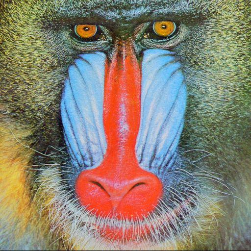
   • mandrill.jpg: Try different parameter values.
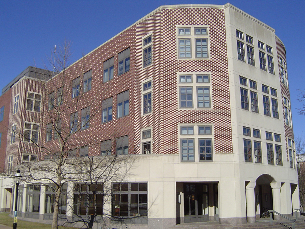
   • csbldg.jpg: Try to find values that will find just the outline of the building, and others that will find edges between individual bricks. Describe all experiments in your writeup PDF file.

Submitting

This assignment is due Thursday, October 3, 2019 at 11:59 PM. Please see the general notes on submitting your assignments, as well as the late policy and the collaboration policy.

As stated, our submissions this year will be done through Gradescope. The code to register for our class and how to submit can be found in the "general notes on submitting..." link above. This assignment has 2 submissions:

1. Assignment 1 Written: Submit one single PDF containing all written portions of the assignments. This contains all work for problems 1-3 (including derivations, plots, and code for problem 3), as well as experiments and findings for problem 4. This portion is worth 60 points (50 points from problems 1-3, 10 points for written portion of problem 4).
2. Assignment 1 Problem 4 Code: Submit your Canny Edge Detection implementation. This should be your version of a1p4_functions.py, where all functions have been filled. Make sure that the filename was not changed, nor were the function names and inputs/outputs. This portion is worth 40 points.

You are expected to use good programming style, including meaningful variable names, a comment or three describing what the code is doing, etc. Also, all images created by your code must be saved with the "cv2.imwrite" function - do not submit screen captures of the image window.

Credit to Fei-Fei Li and Juan Carlos Niebles for several problems.