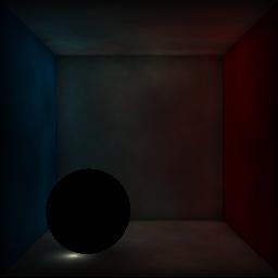
pointlight1.scn
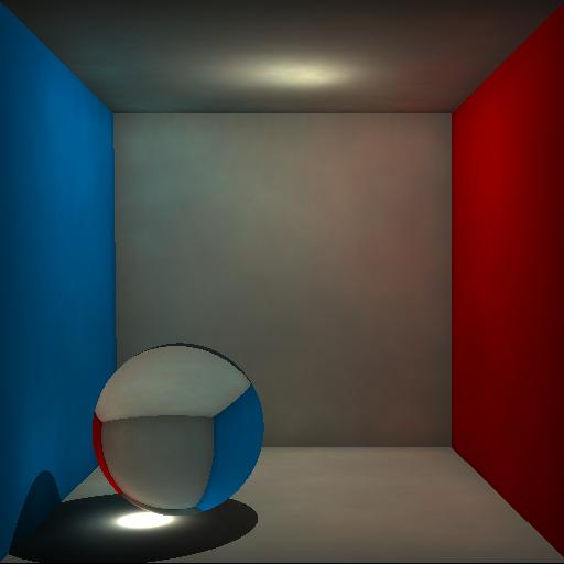
pointlight2.scn
dirlight1.scn
dirlight2.scn
spotlight1.scn
spotlight2.scn
arealight1.scn

arealight2.scn
The flags -nphotons and
-ncaustic_photons control, respectively, the total
number of global photons and caustic photons emitted from light
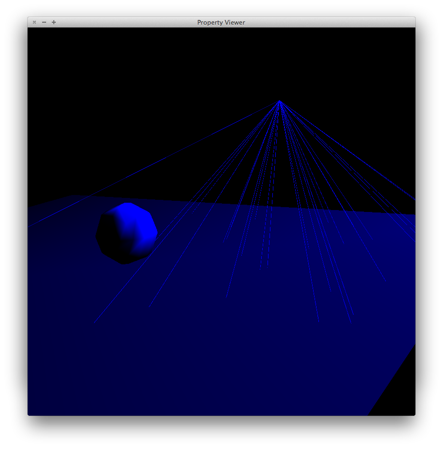
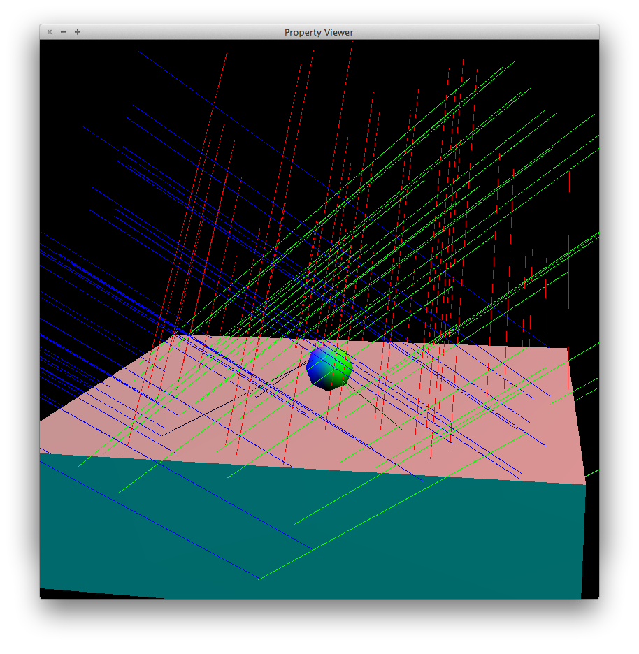
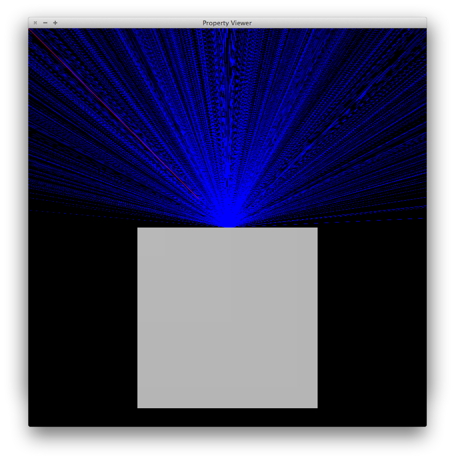
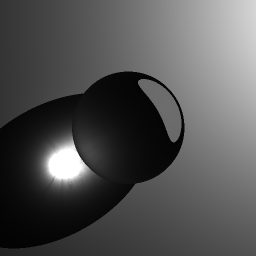
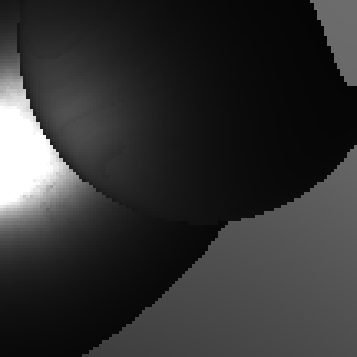
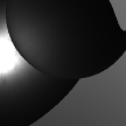
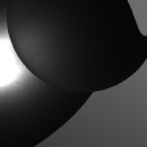
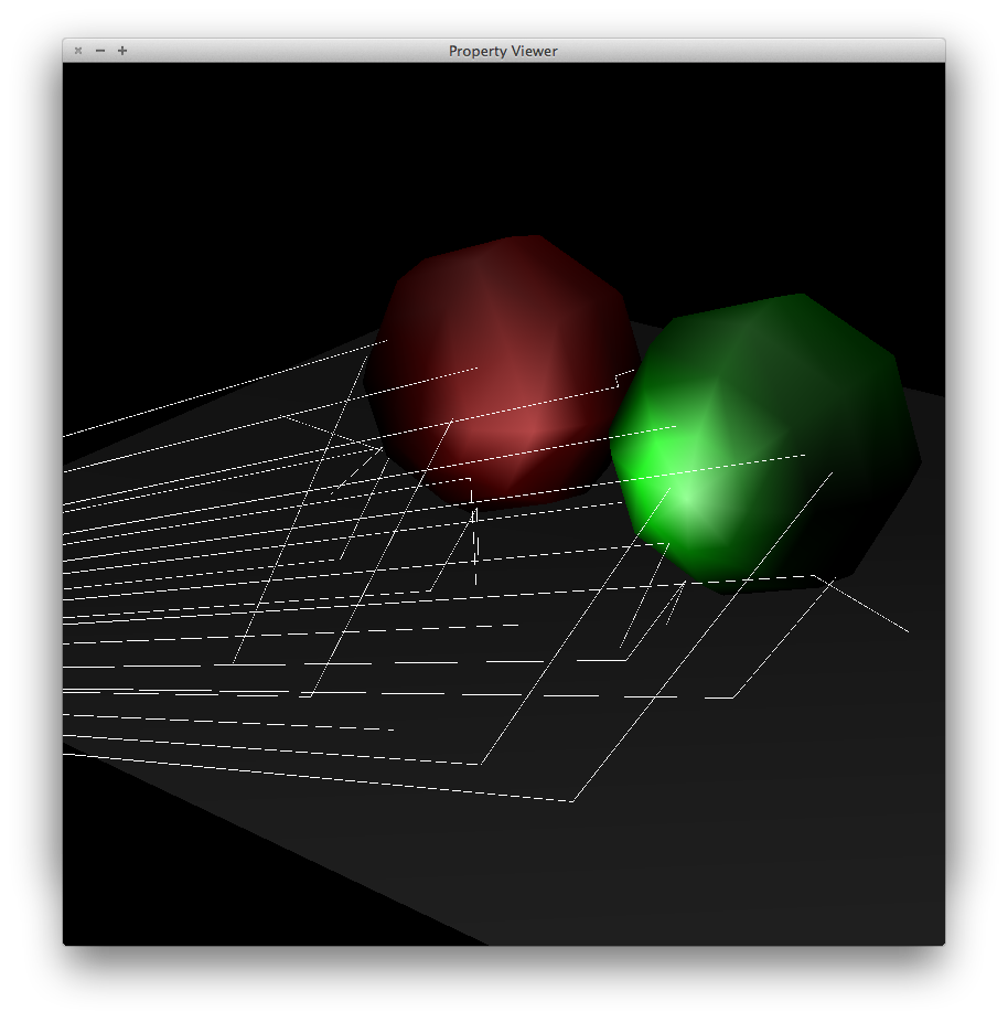
sources in the scene. Point light sources emit uniformly in all
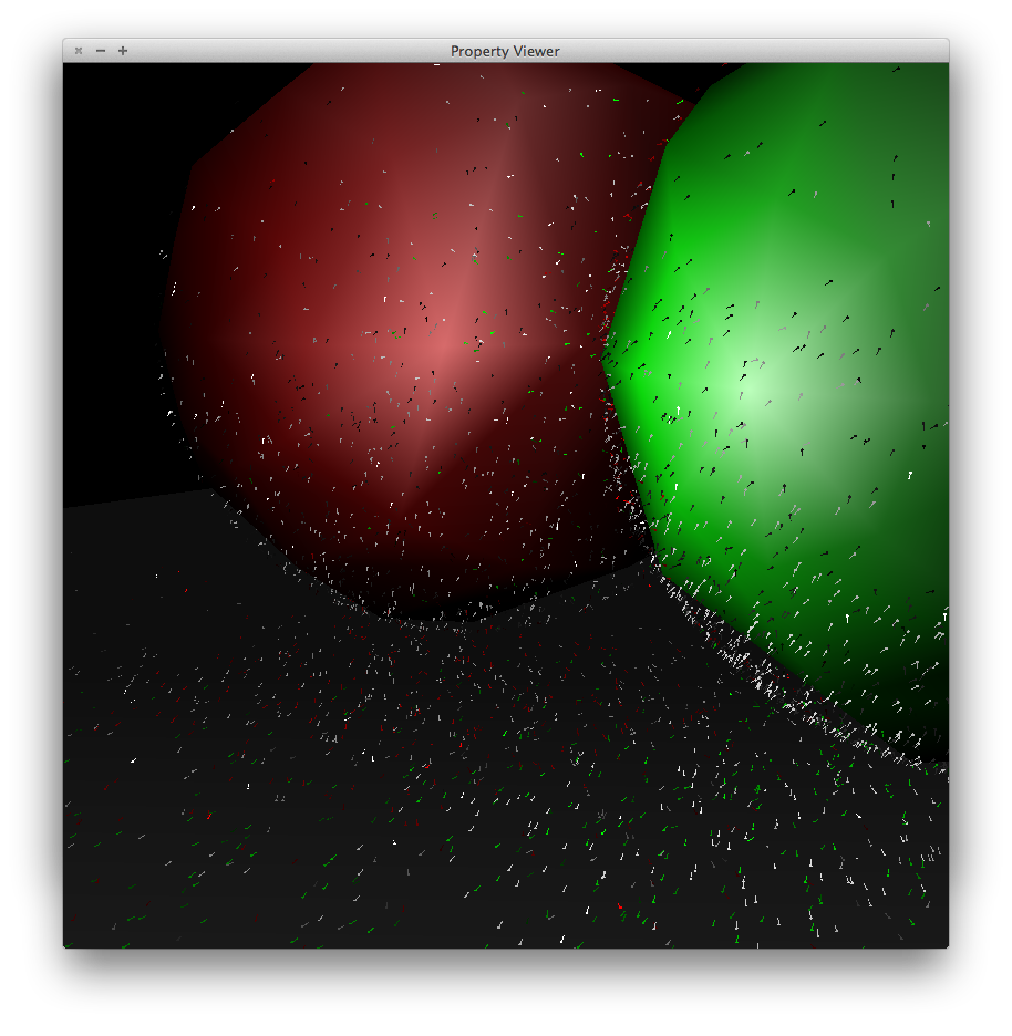
directions. For area light sources, a point is chosen uniformly
at random in the disk, then a direction is chosen in a
distribution weighted by cosine of angle from
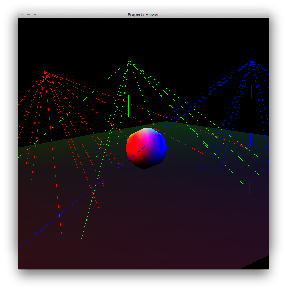
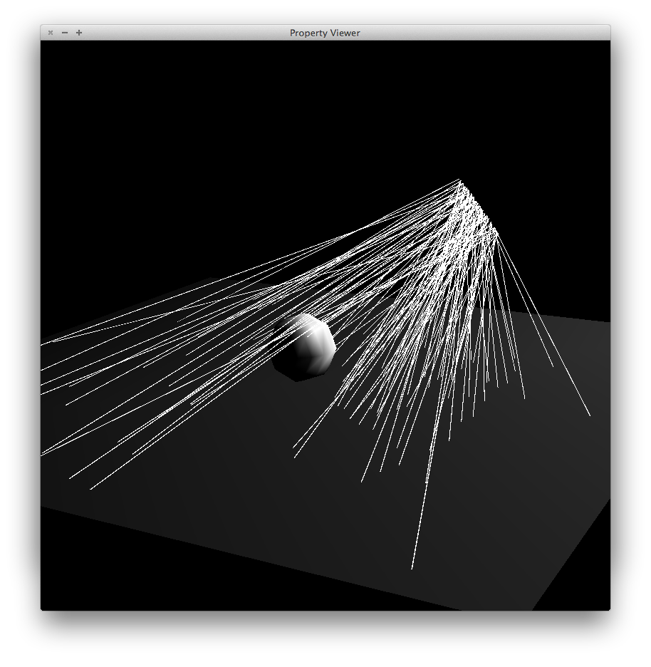
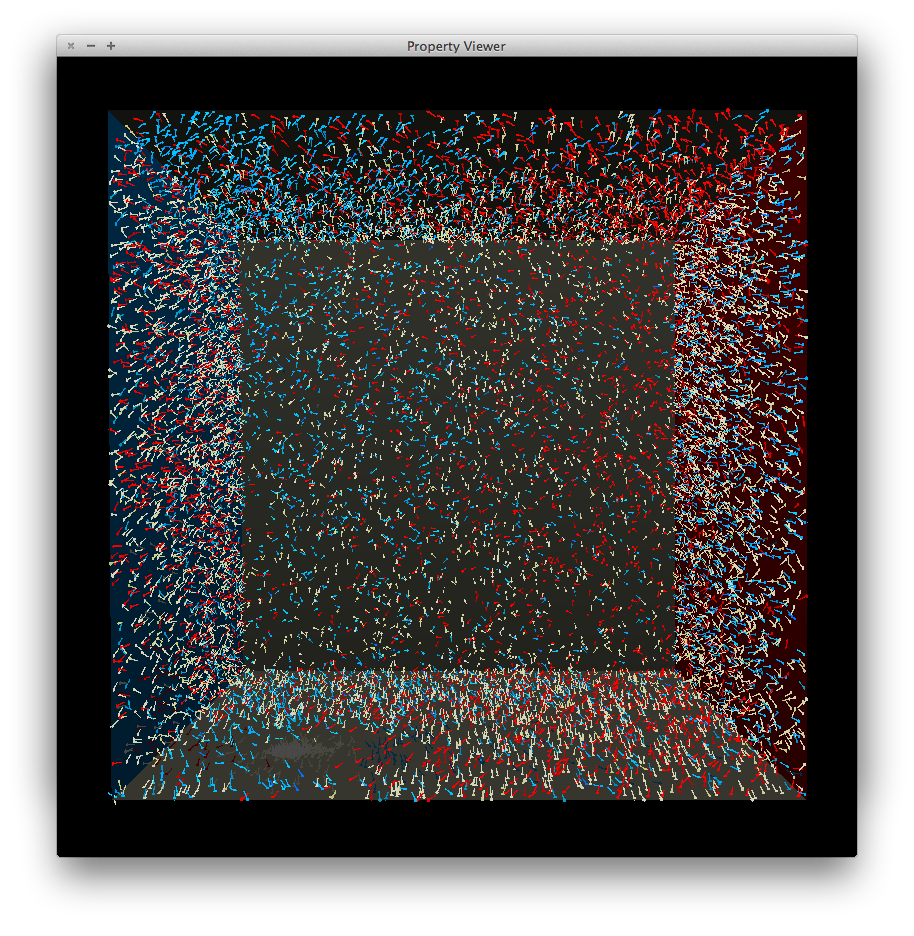
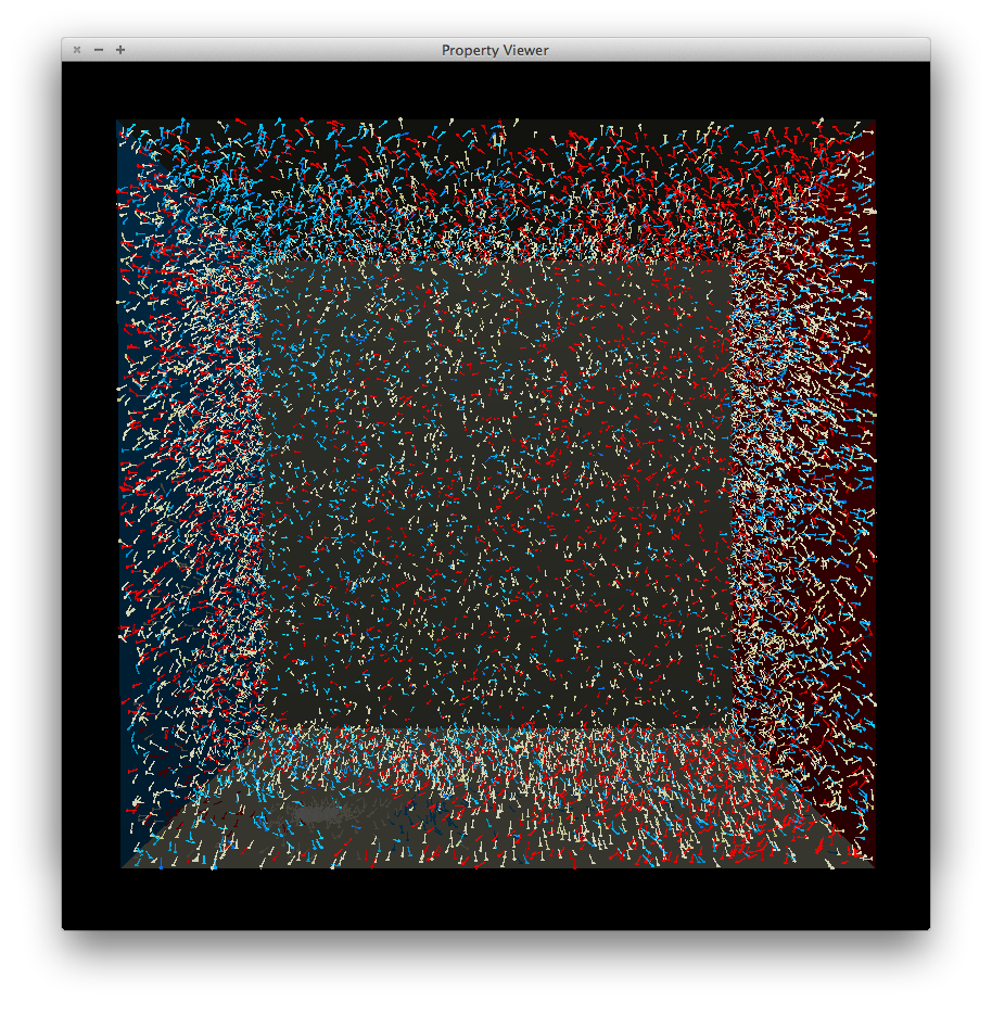
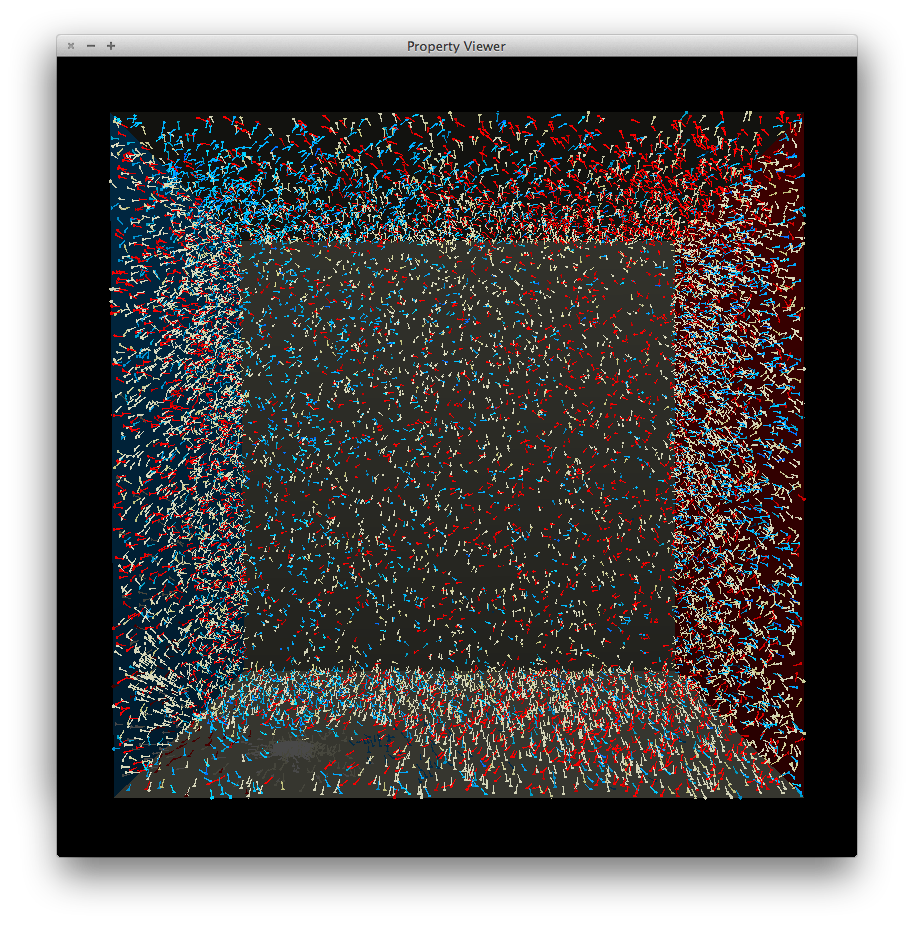
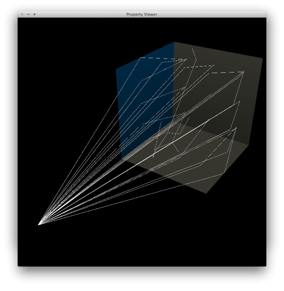
normal. Directional lights shoot photons from a large enough
disk outside the scene, with points chosen uniformly. For
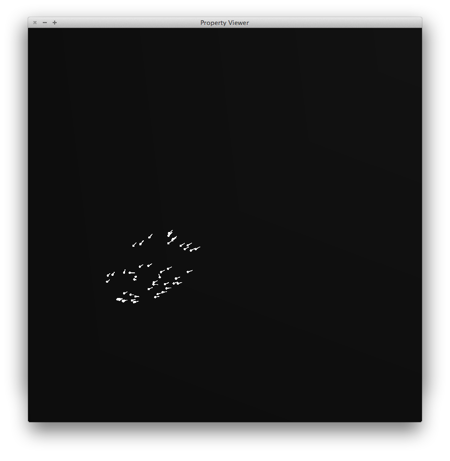
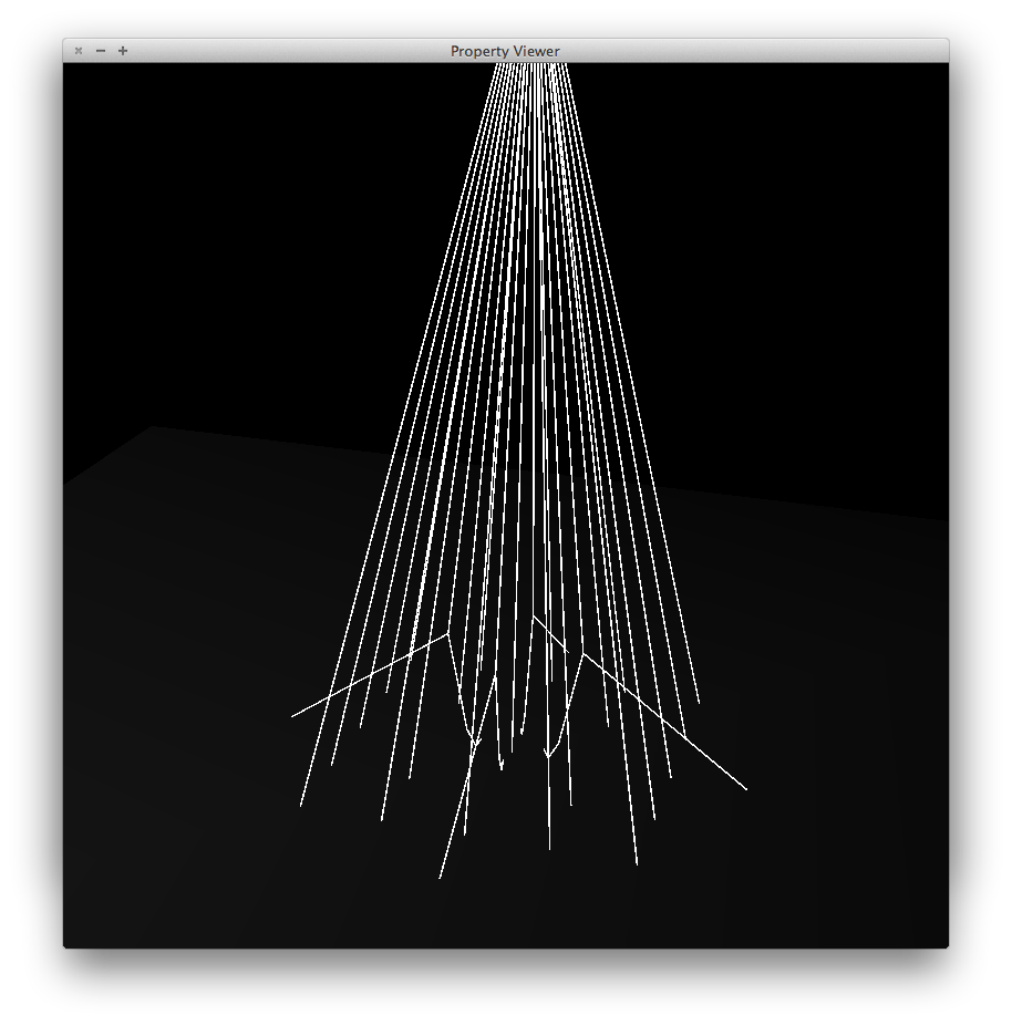
spotlights, the direction is chosen from a distribution similar
to the one described by Jason Lawrence for importance sampling
in specular Phong, with angles outside the cutoff rejected.
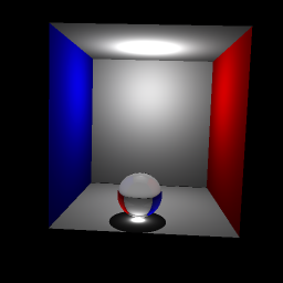
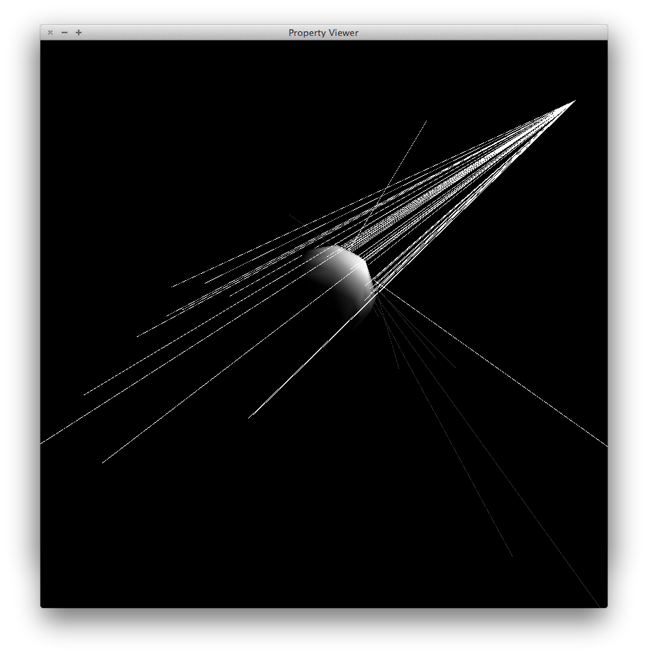
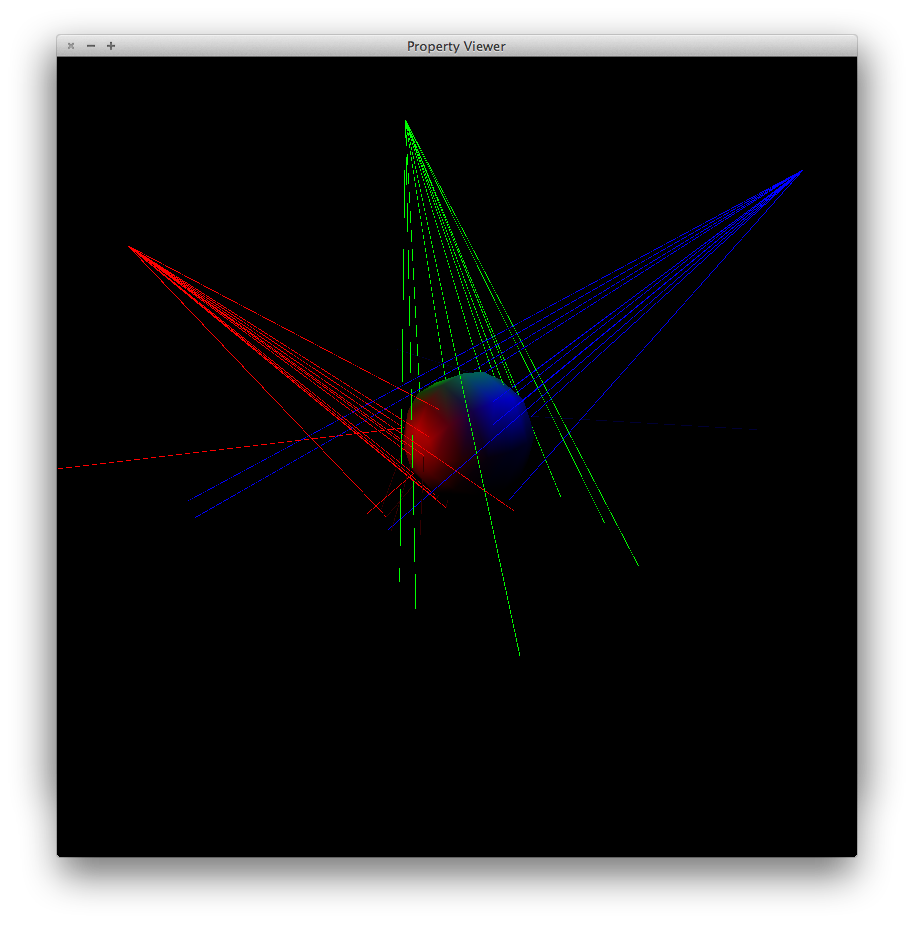
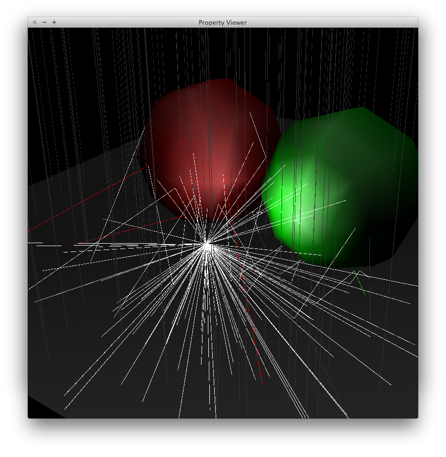
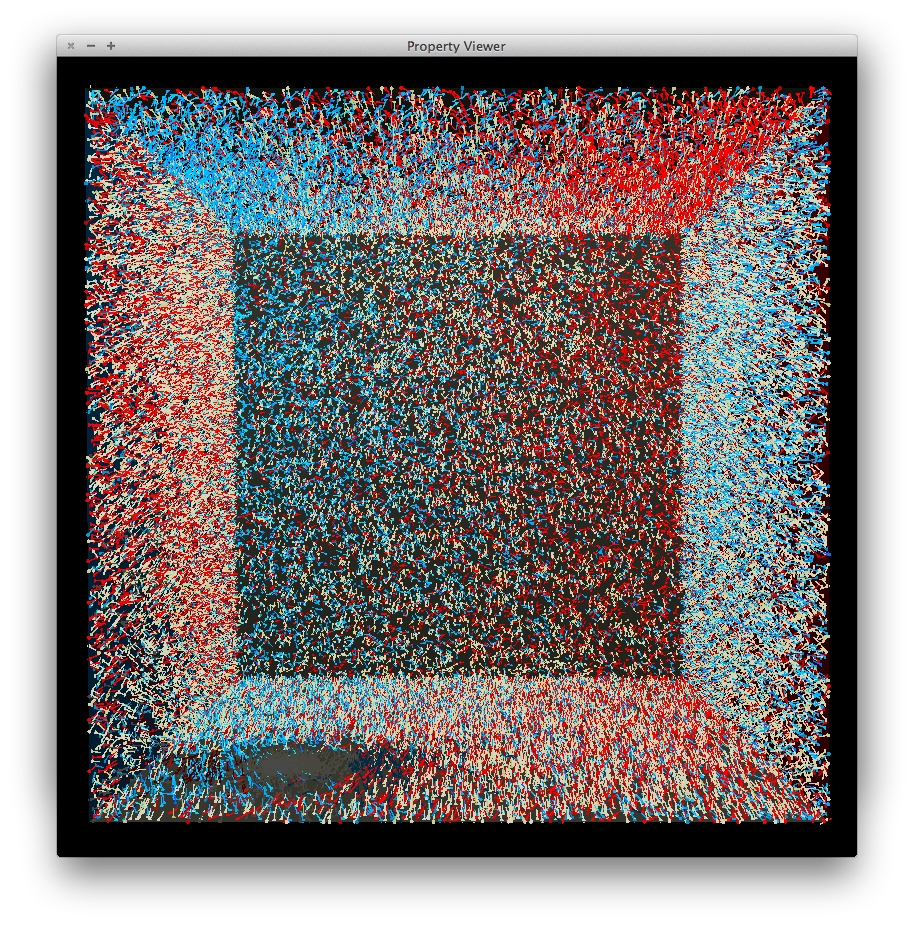
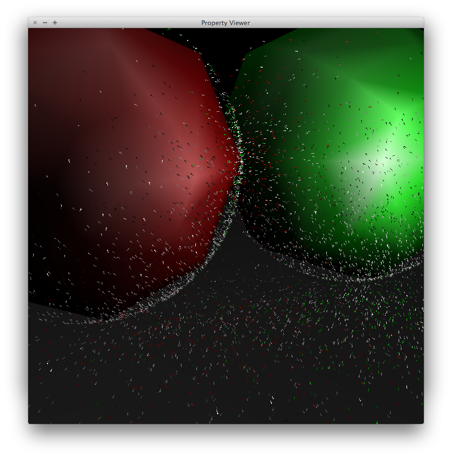
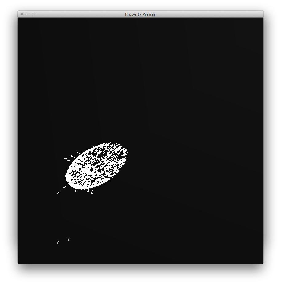
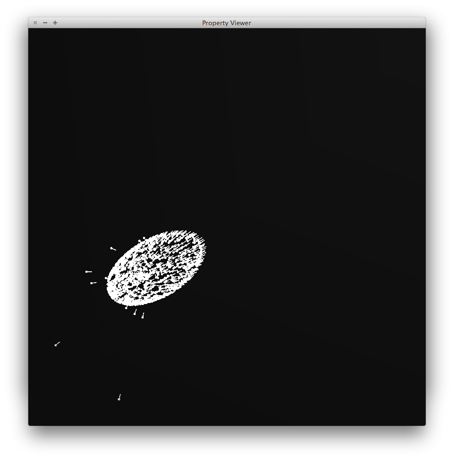
Below are some illustrations. Photon paths are shown by line segments. Only photons that actually hit a surface are shown. Each light type has two illustrations, one with a single light source and another with three light sources of different colors. In all cases the subject is a sphere on a box. At times the lines appear dotted or broken but this is simply due to aliasing in the image -- the actual path is continuous.
|
pointlight1.scn |
pointlight2.scn |
|
dirlight1.scn |
dirlight2.scn |
|
spotlight1.scn |
spotlight2.scn |
|
arealight1.scn |
arealight2.scn |
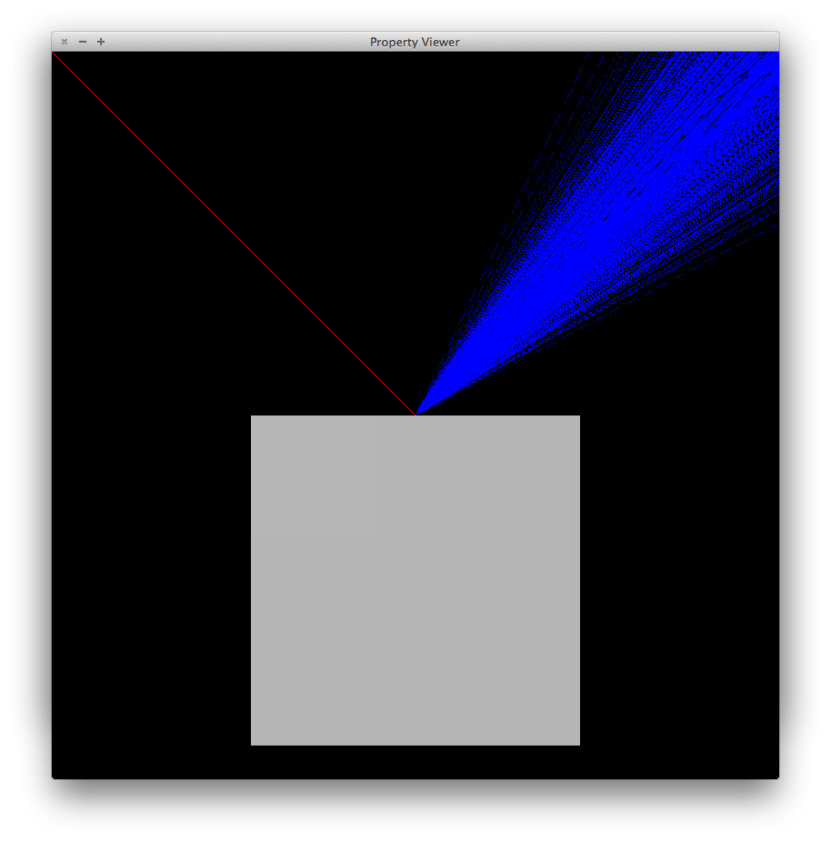
When a photon hits a surface, Russian roulette is used to determine the next step. A secondary ray is shot in either a diffuse, specular or transmission direction, or the photon is 'absorbed' and no secondary ray is shot. The probability of each event is determined by the properties of the material.
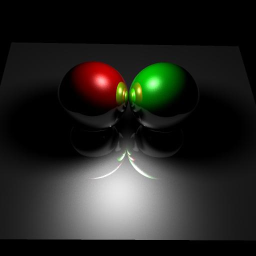
The diffuse and specular scattering distributions are based on Jason Lawrence's notes (BRDF importance sampling). Below an incident direction is shown in red, along which many photons are shot to produce the blue scattered directions.
 Diffuse scattering |
|
 Specular scattering |
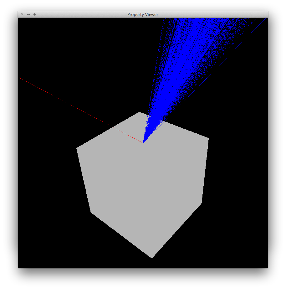 Specular scattering, different viewpoint |
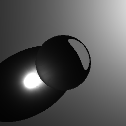
For transmission we just propagate in the single refraction direction. Below a bunch of photon paths are focused into a caustic patch by a transparent ball (the ball is invisible in the image).
|
Transmission |
As this process is repeated, the photons bounce around the scene. Below are illustrations for photon paths up to depth 3 in cornell.scn and specular.scn (the spheres in specular.scn are rendered approximately as low-poly meshes, hence the gaps between their surfaces and the reflection points).
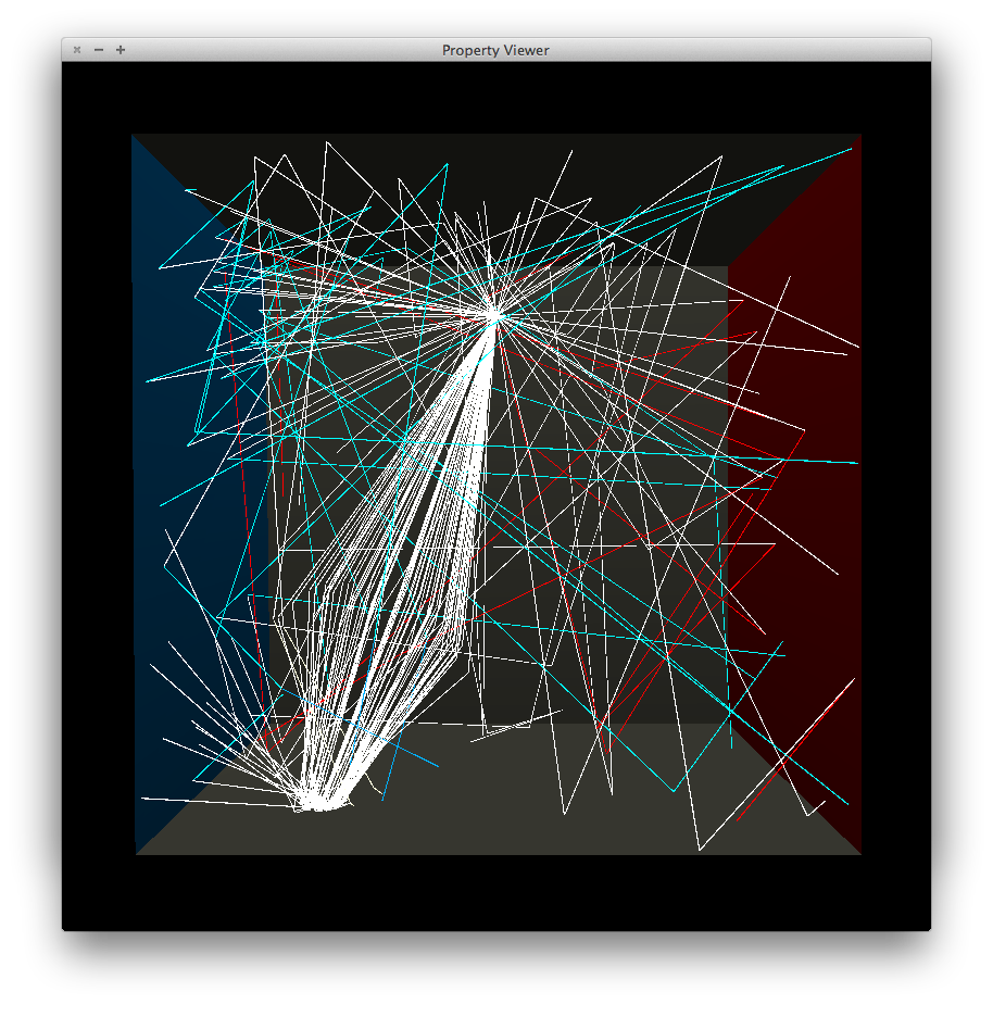 Scattering in cornell.scn |
 Scattering in specular.scn |
Photons are stored in a kd-tree. Their position, direction and power is saved. Below is a visualization of stored photons for some scenes. The photons are visualized with a color slightly brighter than the power actually stored for easier viewing, and have a short tail that indicated the (negative) incident direction.
 cornell.scn (10000 global, 2000 caustic) |
 cornell.scn (50000 global, 5000 caustic) |
 specular.scn (50000 global, 5000 caustic) |
 specular.scn (100000 global, 10000 caustic) |
Two separate photon maps are generated, in separate passes. One is the usual global photon map, the other is the caustic photon map for which the first bounce must be a specular reflection or a transmission. The number of photons generated for each can be varied separately.
 cornell.scn (global photon map) |
 cornell.scn (caustic photon map) |
 cornell.scn (both) |
 caustic.scn (global photon map) |
 caustic.scn (caustic photon map) |
 caustic.scn (both) |
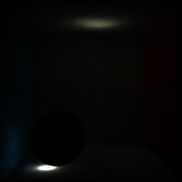
To produce the final image, rays are traced from the camera. At each surface intersection, the direct illumination (check shadow ray, then do a phong lighting calculation), specular/transmission (trace secondary rays), caustic (use the caustic photon map) and indirect illumination (use the global photon map) contributions are computed and combined.
Here are some illustrations of each part in cornell.scn:
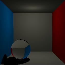 cornell.scn (direct, specular/transmission) |
 cornell.scn (caustics) |
 cornell.scn (indirect) |
And here is the final render, combining all parts:
 cornell.scn (all) |
Some other scenes:
 caustic.scn |
 softshadow.scn (with 4 rays per pixel, see below) |
Multiple rays are shot through each pixel for raytracing (following a grid pattern per pixel), then the results are averaged to give the final color of the pixel. Below is a comparison at various multiplicities:
 1 ray per pixel |
 4 rays per pixel |
 9 rays per pixel |
Zoomed in:
 1 ray per pixel |
 4 rays per pixel |
 9 rays per pixel |
-viz_rays option. Below are
illustrations of rays traced in the cornell.scn, specular.scn
and caustic.scn scenes.
 cornell.scn |
 specular.scn |
 caustic.scn |
The given R3Kdtree class uses a naive sorted
array to collect the N closest points asked for. I implemented
an alternative member function, FindClosestQuick()
which uses a max-heap instead (as provided by
std::priority_queue in the C++ standard
library). This is suggested on page 35 of the jensen01
reading. Further, I made an optimization that assumes that the
position field of R3Kdtree elements is at the
beginning of the struct, which eliminates the need for a
callback function or for offsets (effectively, the offset
becomes zero).
This provides a considerable speedup. The render time of the
following scene was reduced from 21.30 seconds (using the given
R3Kdtree) to 10.01 seconds (using my optimized
method).
For comparison, the optimization can be turned off by
providing the -slow_kdtree option to
photonmap.
 caustic.scn |
I made a short video of a scene that looks like the cornell box, with the glass sphere starting in the air, fall onto the floor then rolling to the side (the box is slightly tilted). The animation was made with Blender. The frames were exported to .scn using the scn_export.py plugin for Blender which is included as art/scn_export.py.
Each frame scene is also already provided as frame1.scn, frame2.scn and so on till frame250.scn under the art/ directory. The rendered frames are also provided as .bmp files. The frames were stitched together to produce the final video, art/art.mp4.
Here is a link to the video.
Here is a screenshot from the video: