
|
|
COS 429 - Computer Vision |
Fall 2016 |
| Course home | Outline and Lecture Notes | Assignments |
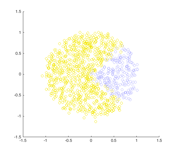
The "network" that you trained in part 1 was rather simple, and still only supported a linear decision boundary. The next step up in complexity is to add additional nodes to the network, so that the decision boundary can be made nonlinear. That will allow classifying datasets such as this one:
We will implement a really simple network with a single "hidden layer" – that is, one layer of computation that isn't an input or output – with two nodes. Here is the architecture that we will use:
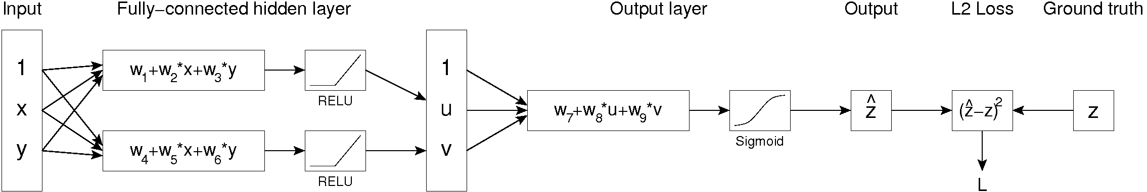
For convenience, we've given the names $u$ and $v$ to the outputs of the two hidden nodes, and $\hat{z}$ to the final output. As before, $z$ is the ground-truth label. The different $w$ are the weights to be learned during training, then used during testing. (In the code, the vector of $w$ is called params.)
To train this network using SGD, we need to evaluate $$ \nabla L = \begin{pmatrix} \frac{\partial L}{\partial w_1} \\ \frac{\partial L}{\partial w_2} \\ \frac{\partial L}{\partial w_3} \\ \vdots \end{pmatrix} $$
As discussed in class, evaluating these partial derivatives is done using "backpropagation", which is just a fancy name for repeatedly applying the chain rule of differentiation. For example, suppose we wish to evaluate $\frac{\partial L}{\partial w_5}$. Tracing back through the network to find the dependency, we know that $L$ depends on $\hat{z}$, which depends on $v$, which in turn depends on $w_5$. So, using the chain rule, we can write $$ \frac{\partial L}{\partial w_5} = \frac{\partial L}{\partial \hat{z}} \frac{\partial \hat{z}}{\partial v} \frac{\partial v}{\partial w_5} $$ and then proceed to write out all of those partial derivatives: $$ \frac{\partial L}{\partial w_5} = \bigl( 2 \; (\hat{z} - z) \bigr) \bigl( \hat{z} \; (1 - \hat{z}) \; w_9 \bigr) \bigl( Z(v) \; x \bigr) $$ Here $Z$ is a function that returns 1 if its argument is $>$ 0 and 0 otherwise. (Note that it's critical for this to be defined as $>$ 0 and not $\geq$ 0.) $Z$ is the derivative of RELU, just as $\hat{z}\;(1-\hat{z})$ is the derivative of the sigmoid.
In order to understand the computation, we strongly suggest that you write out the partial derivatives of $L$ with respect to all the weights, and understand their common components. In particular, you should not multiply out the expressions for the partial derivatives - for efficient computation, you should re-use as many common subexpressions as possible.
The starter code for this part defines a function tinynet_sgd that supports the above architecture, except with an input vector of arbitrary dimensionality (and explicitly including the constant "1" as the first element of the input vector). Therefore, it will require $2d+3$ weights, where $d$ is the dimensionality of each data point. There are $d$ weights for each of the two hidden nodes, plus 3 weights for the final output node. Think about how you can structure the computation of the complete $2d+3$ dimensional gradient using a set of dot products against the datapoint.
Do this:
Download the starter code for this part.
It contains the following files:
Modify tinynet_sgd.m to compute the gradient, and to train the network using SGD. Run test_tinynet several times - you should see the network converging to a correct result some, but not all, of the time.
Modify test_tinynet to re-run the training multiple times. What fraction of the time does the training converge to a good (> 95% correct) result? Does this vary appreciably with the number of SGD iterations (i.e., num_epochs)? How about with different learning rates?