Advanced Computer Graphics' 2nd Assignment by Thiago Pereira
Overview
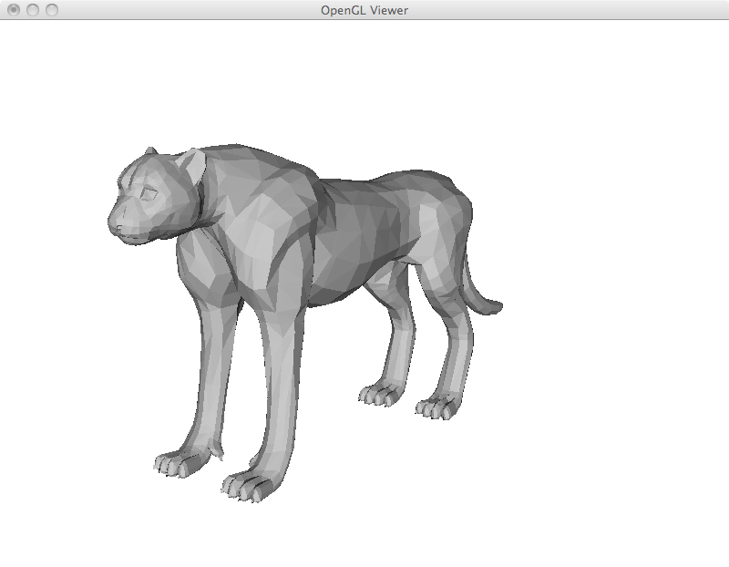
In this assignment, I implement and explore different applications of Laplacian Meshes. In this representation, instead of representing a vertex by its cartesian coordinates, we store Laplacian coordinates. This is a representation where each vertex is stored relative to its neighbors. By manipulating this coordinates and reconstructing a mesh a number of different operations can be implemented such as deformation, parametrization, membrane filling, function interpolation and curvature computation.
Features
Basic Laplacian mesh representation
I calculate the Laplacian matrix based on the topology and geometry of the mesh by using cotangent weights. We can obtain the Laplacian coordinates by multiplying the matrix by a vector with the cartesian coordinates. More specifically, I multiply by 3 vectors for x, y and z. All the linear algebra operations in this assignment were done using the CSparse library. After, the Laplacian matrix and coordinates are computed, they no longer change during the execution of the program. This means I store the details always relative to the first mesh. Alternatively, one could update them after each operation or periodically.
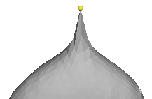
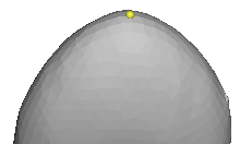
Mesh Reconstruction
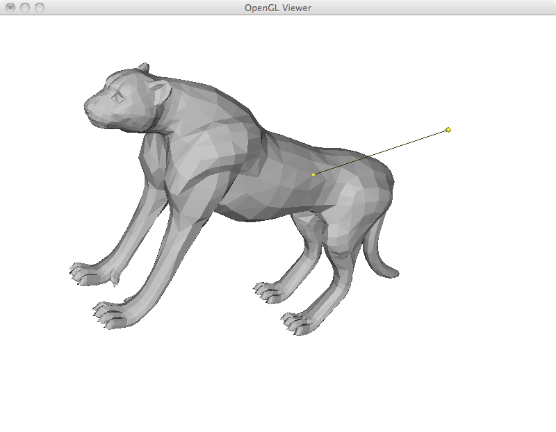
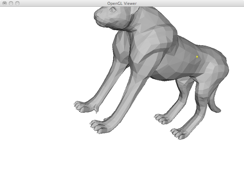
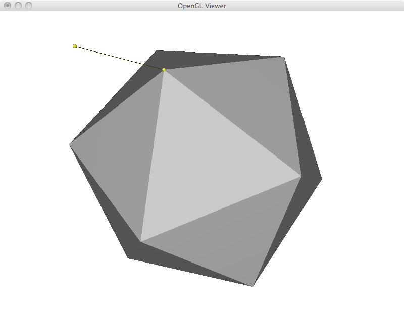
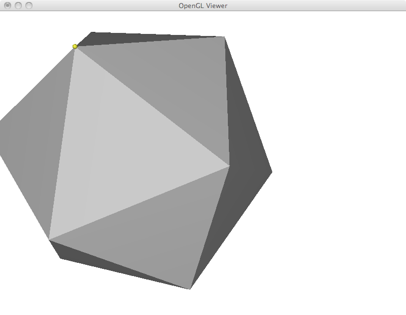
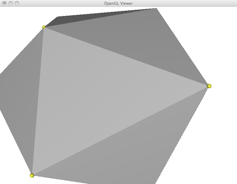
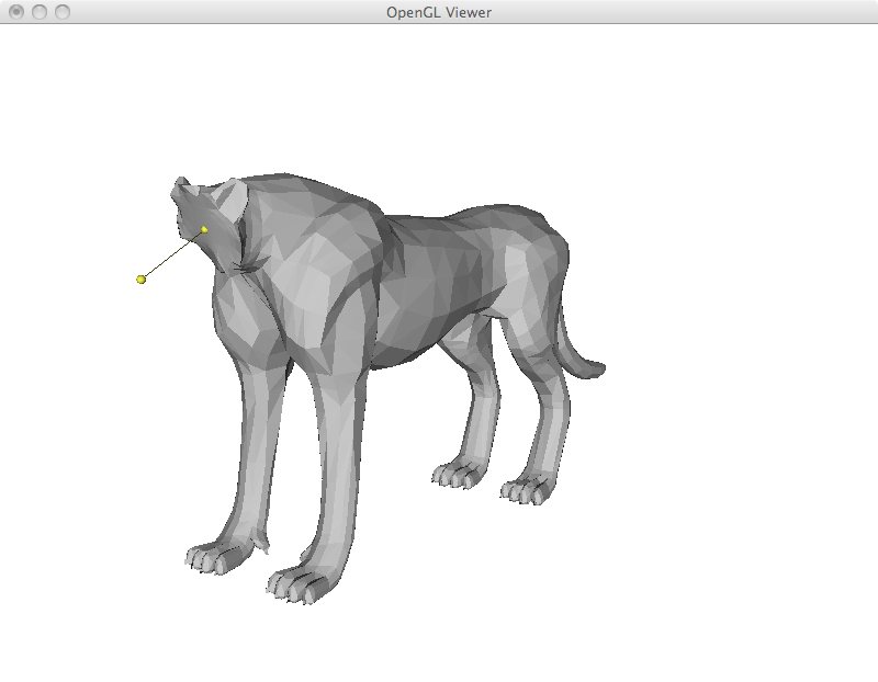
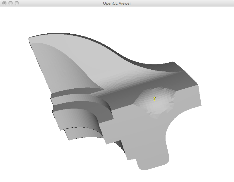
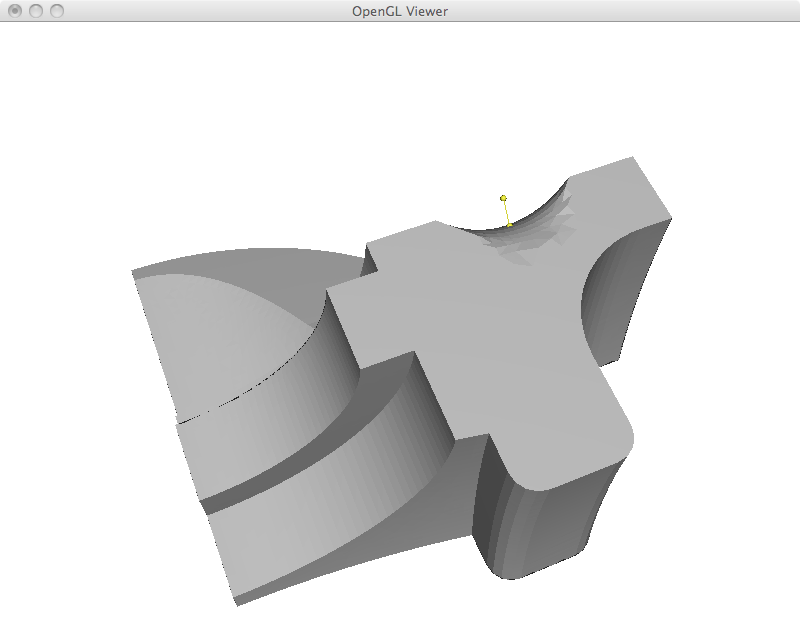
Most operations in the next sections are based on an overall framework. We first compute the Laplacian coordinates, we manipulate them and finally we reconstruct cartesian coordinates from them. In its most basic formulation, I implemented the mesh reconstruction step by adding a new row to the matrix to restrict the position of a given vertex. Computationally, all linear systems in this assignment were solved in the least squares sense by explicitly building the A^T A matrix and using the Cholesky factorization. However, the resulting system often results in zero residual. This is the case in this section, where the extra equation is only added to complete the rank. In the examples that I show below, the yellow vertex is moved to a new position and the whole mesh is reconstructed. This results in a translation of the matrix with perfect preservation of its shape. As a final efficiency remark, this implementation could be made much faster by storing the factorized matrix and reusing it. In its current form, I am refactorizing the linear system each time.
Mesh Deformation
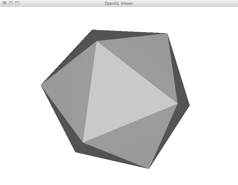
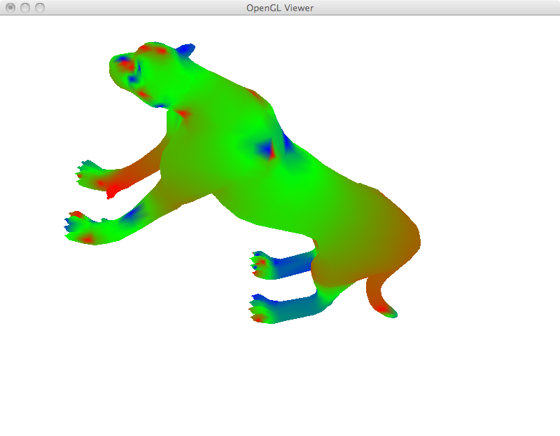
For mesh deformation, I simply add the fixed point restrictions as new rows in the Laplacian matrix. A weight of 1000 is given to these equations, as such they are exactly satisfied. Up to this point, all restriction are specified by the user including deformed points and points that are fixed in place. I begin with a simple example of moving three points of an icosahedron. While the overall shape is preserved, the icosahedron was stretched to satisfy the user constraints.
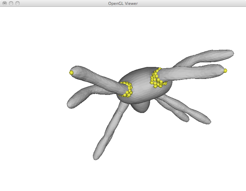
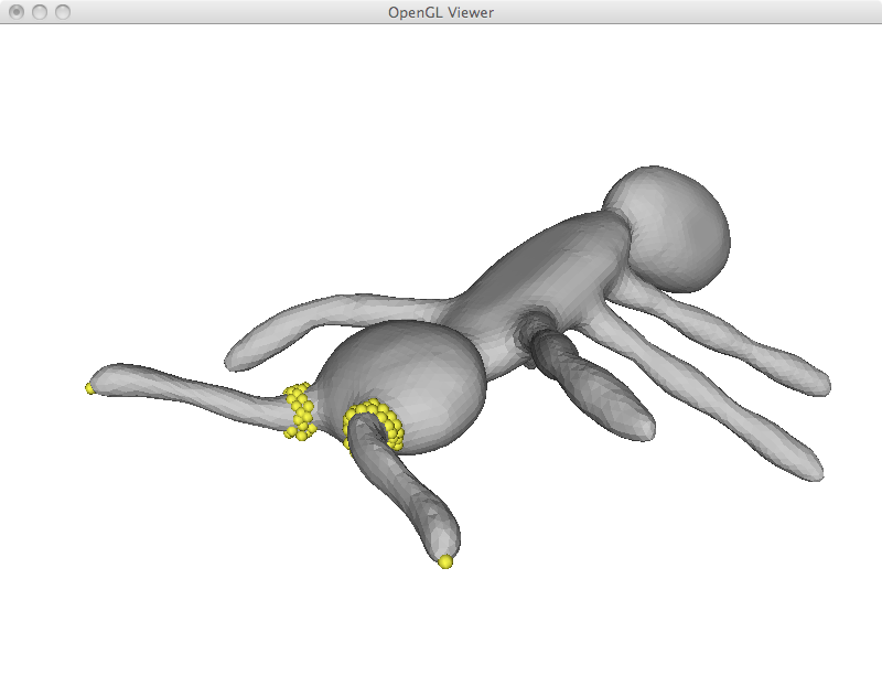
While I implemented simple region of interest control later on, it is already possible to emulate this behavior by adding a large number of fixed points and using another one as a handle. This is specially useful to deform limbs and give the appearance of articulated motion. However, simply solving the Laplacian system has its limitations as can be seen in the last ant image. In this example, its antlers were extremely compressed and became very thin.
Preserving the original Laplacian coordinates in the least squares sense does a very good job at preserving the details. In particular, as can be seen below, even very sharp features are well preserved after deformation.
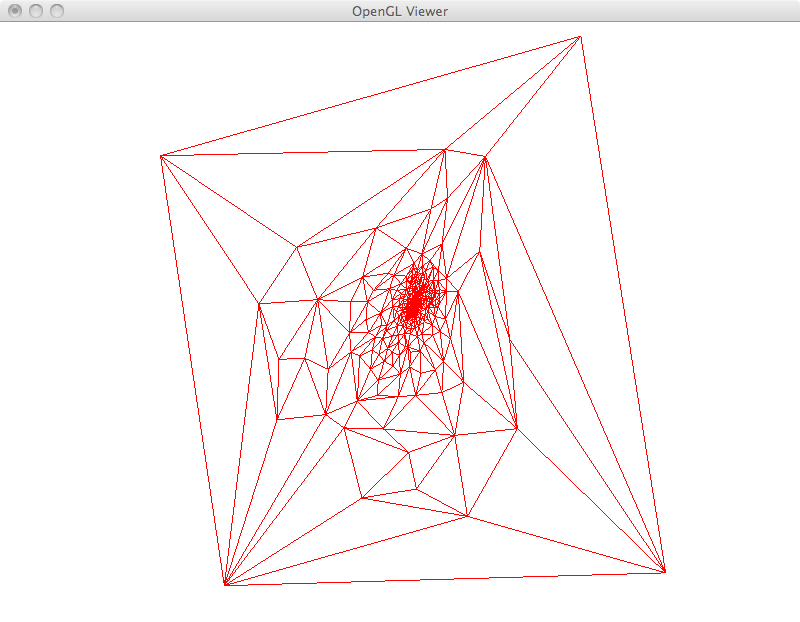
Parametrization
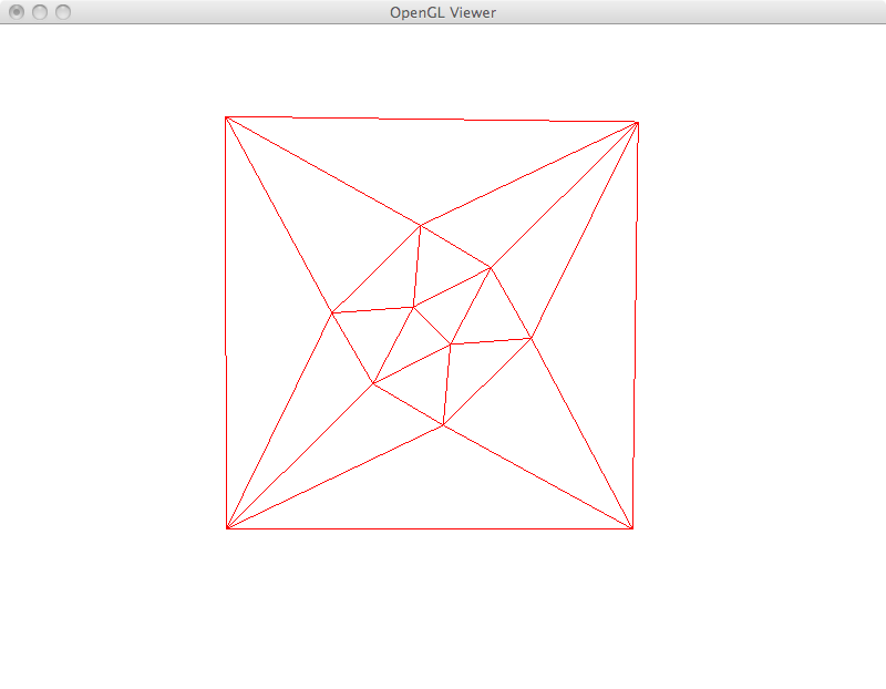
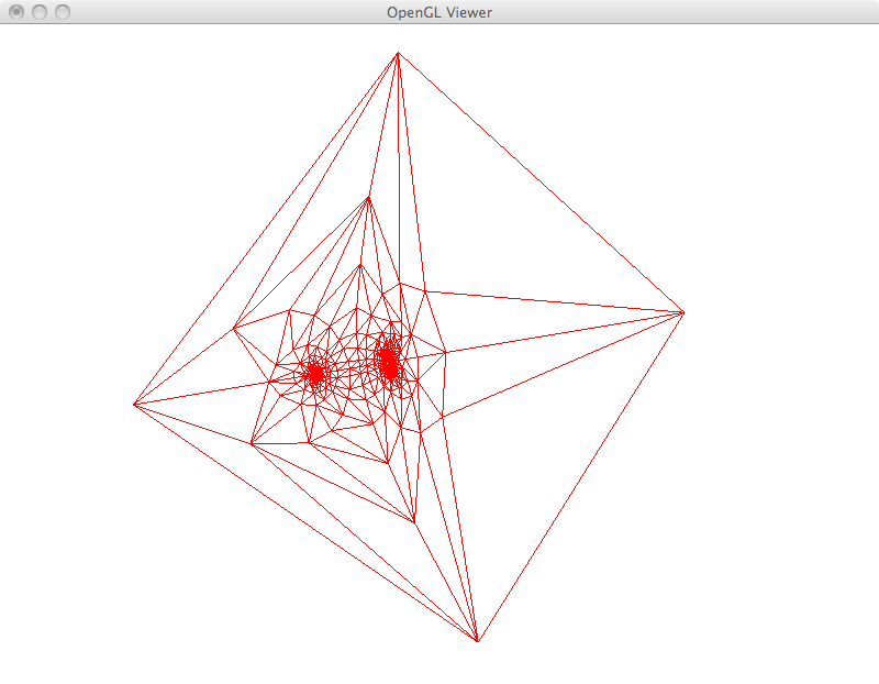
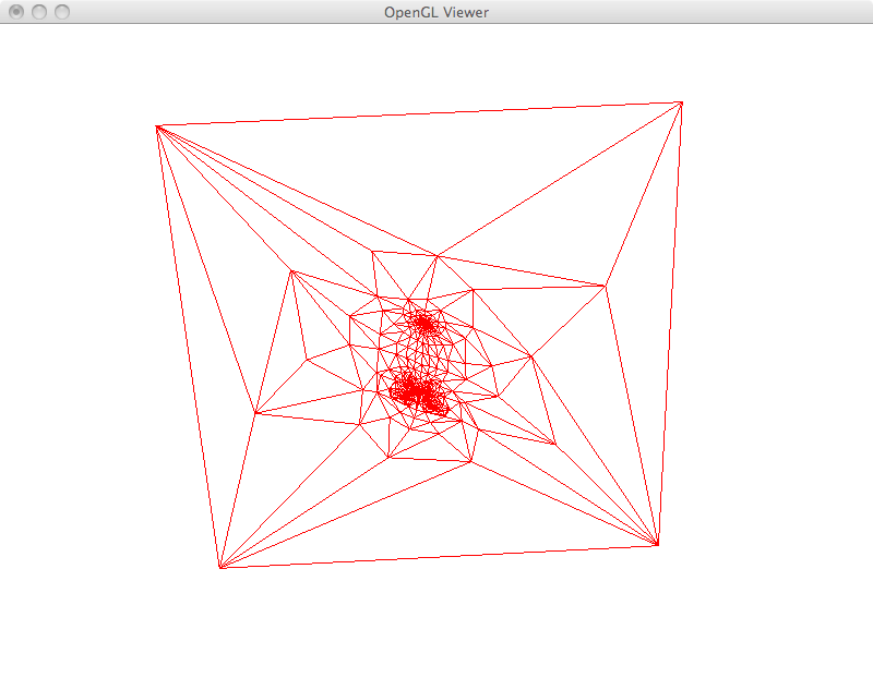
For mesh parametrization, I adapted the user interface to input two vertices as a way of selecting an edge. This edge together with its two neighboring faces are removed from the mesh and the four associated vertices are mapped to the boundary of a unit square. The remaining positions are solved by setting the Laplacian to zero for all the remaining vertices. For this task, besides adding the four vertex constraint rows, I also filled the Laplacian equations corresponding to these vertices to zero. This is equivalent to removing these equations, but was simpler to implement. If removing or zeroing out is not performed, a few mesh vertices may fall outside the unit square.
Below I show examples with the icosahedron and with the cheetah. In the case of the cheetah, three different cuts were performed in its back, belly and nose. However, the quality (or lack of) of the resulting parametrization is similar for all of them. The main problem is that hooking a very small area, in this case only two triangles wide to the border of the square introduces huge distortions. All the rest of the mesh has to find its place inside the square. A better approach would be to have a bigger cut with more vertices and hook this along the square boundary. These unit squares are being visualized inside the 3D canvas creating perspectively distorted images.
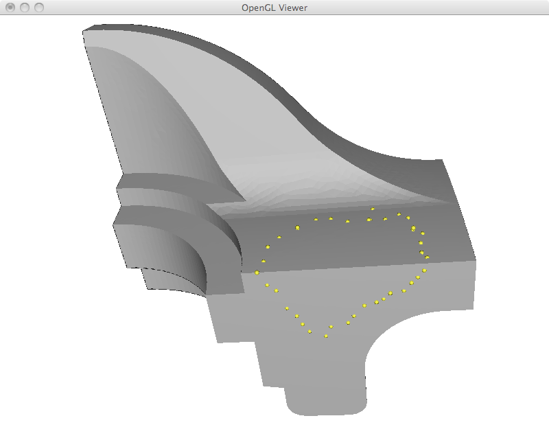
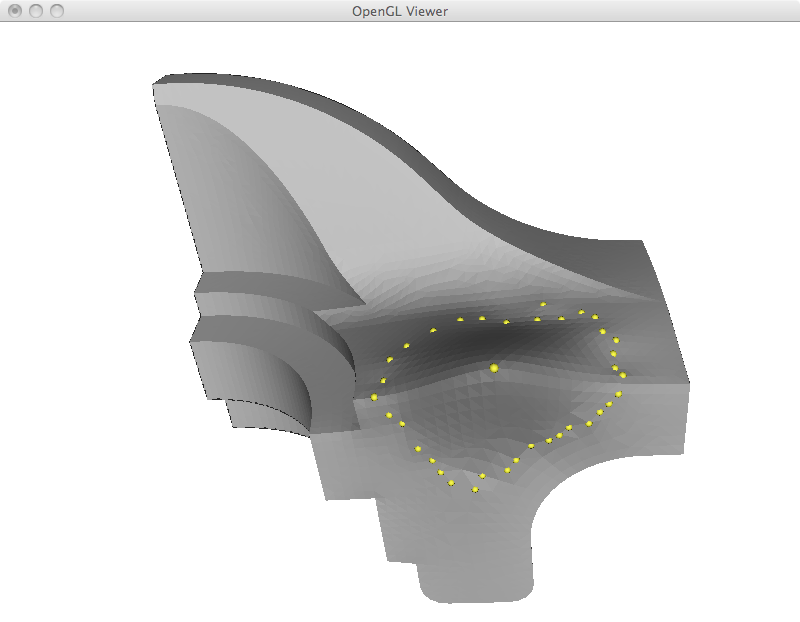
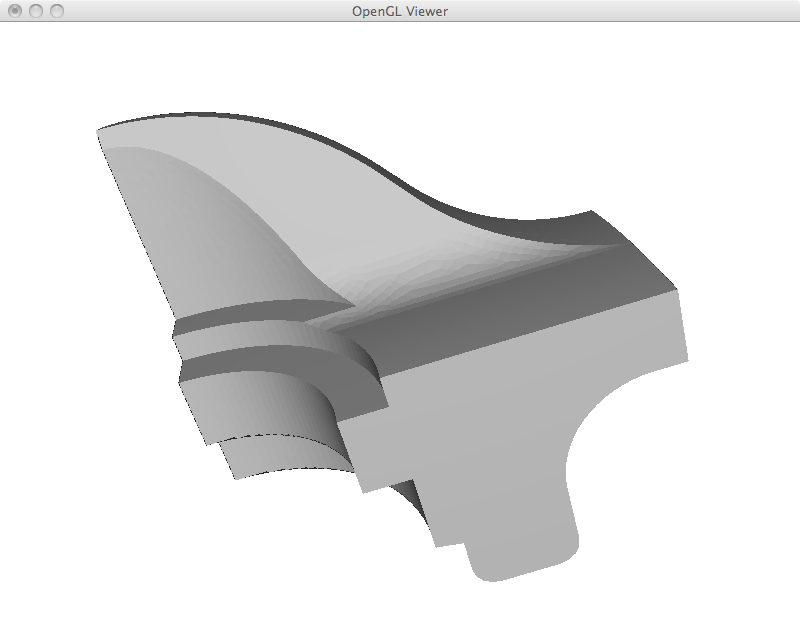
Membrane surface
In this section, I implemented a region of interest scheme to select a few points as boundary conditions that are going to stay in place. All the points inside the region had their Laplacian coordinates set to zero, such that when we reconstruct we get a very smooth interpolant between the boundary points. By very smooth, I mean the resulting surface is going to have zero mean curvature inside the membrane. The reason we can achieve this zero error in the least squares is because we remove (by zeroing the corresponding rows) the laplacian restrictions on all the fixed points. The result is mathematically equivalent to an NxN matrix, although computationally we are still doing least squares. Worse results were obtained when I did not remove this restrictions.
The way I implemented the region of interest control is by calculating a distance field using Dijkstra's algorithm. The user selects the center of the membrane and the points at approximately a fixed radius of this vertex become boundary conditions.
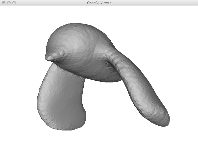
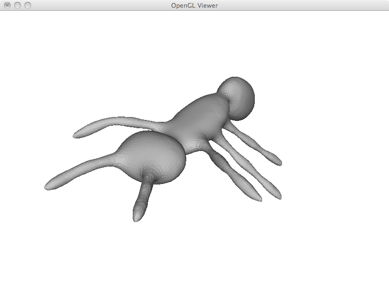
We show some results on the fan model below. These examples show some interesting characteristics of this membrane filling strategy. First, since the Laplacian effectively does averages, it can be seen that all the points inside the membrane are actually inside the 3D convex hull of the boundary points. Second, this examples show how membrane filling can be used to remove features of the mesh. For example by selecting a thin region around a sharp edge and replacing it by a smooth interplant.
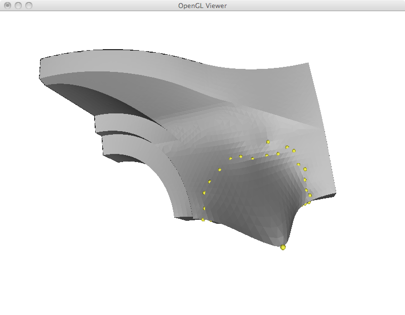
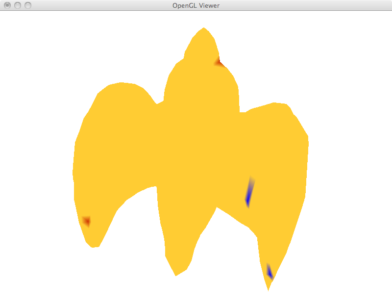
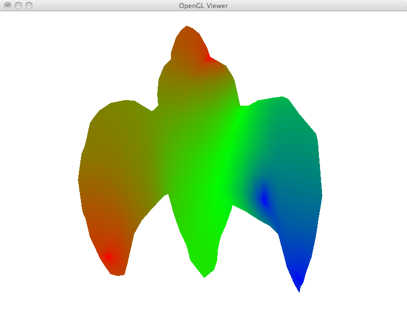
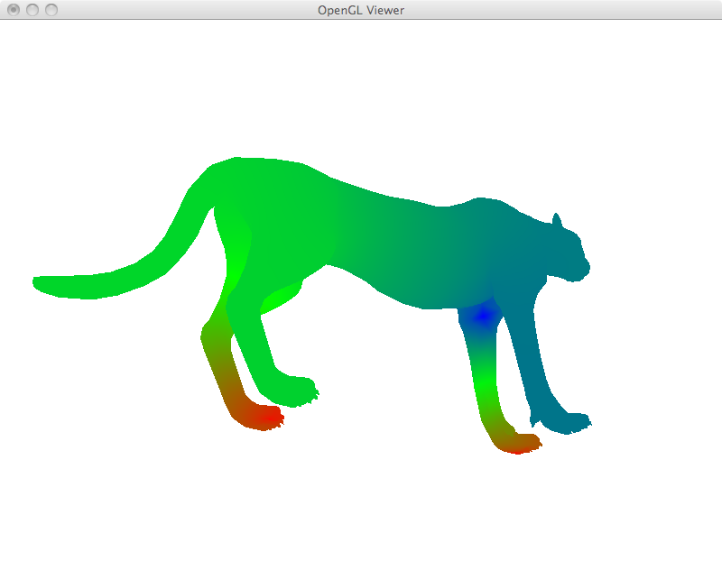
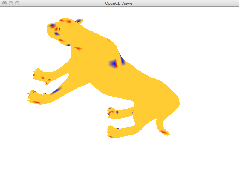
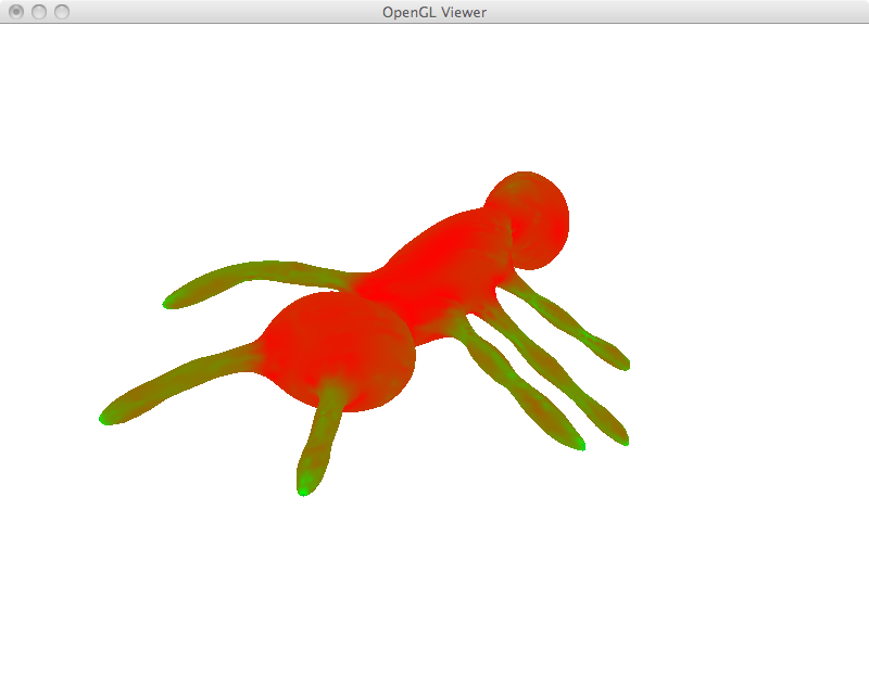
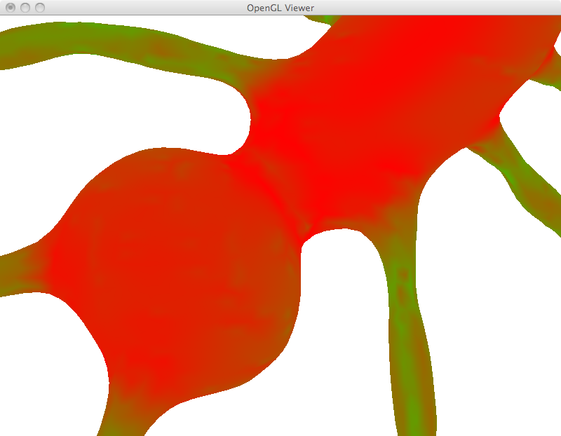
Function interpolation
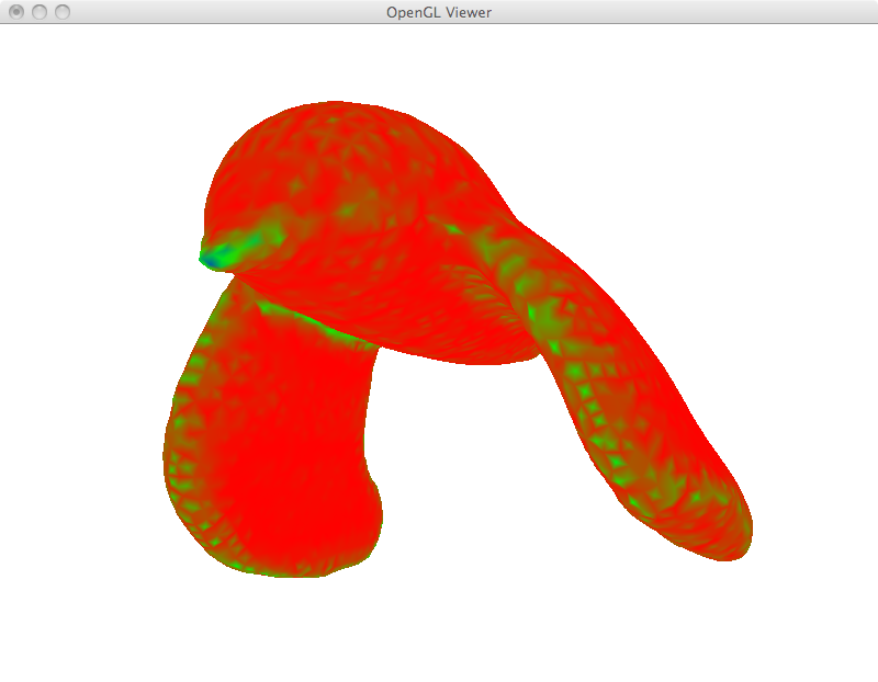
Similar to the membrane case, we can solve Laplace's equation for interpolation of any other function on the mesh, not only positions. We set the Laplacian to zero everywhere, except for a fix set of given points where we only set values. In the examples below, red and blue values were set to specific vertices and interpolated across the mesh. Once again the again the averaging powers of the Laplacian, also known as the maximum principle, lead to many average values on the mesh (shown in green) and few extreme values only on the restrictions themselves (shown in saturated red and blue). In the images below, yellow shows empty vertices before interpolation.
Mean Curvature
It is easy to calculate mean curvature from the Laplacian coordinates. In fact, the Laplacian vector itself is actually a vector in the direction of the normal whose length is twice the mean curvature. As such, we just take its length at each vertex and divide by two.
In the bird example below, I took the bird mesh, subdivided and smoothed it a few times before calculating curvature. However, we still get noisy estimates since the Laplacian is a one-ring estimator. Estimators that use bigger neighborhoods should be able to provide smoother curvature. The ant example below shows an interesting characteristic of mean curvature. Even though, we would intuitively attribute higher curvature to places like the neck, in fact we get some very low values (light red). The reason is in this region we have positive and negative principal curvatures canceling each other out.
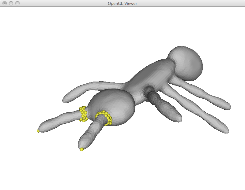
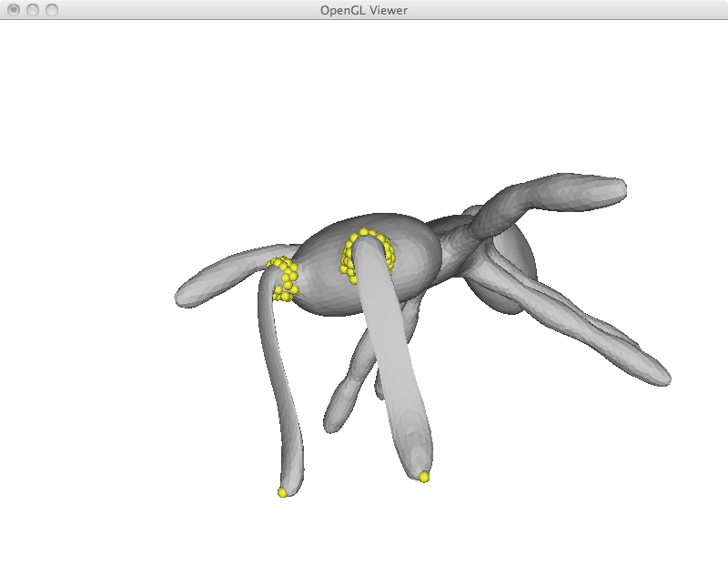
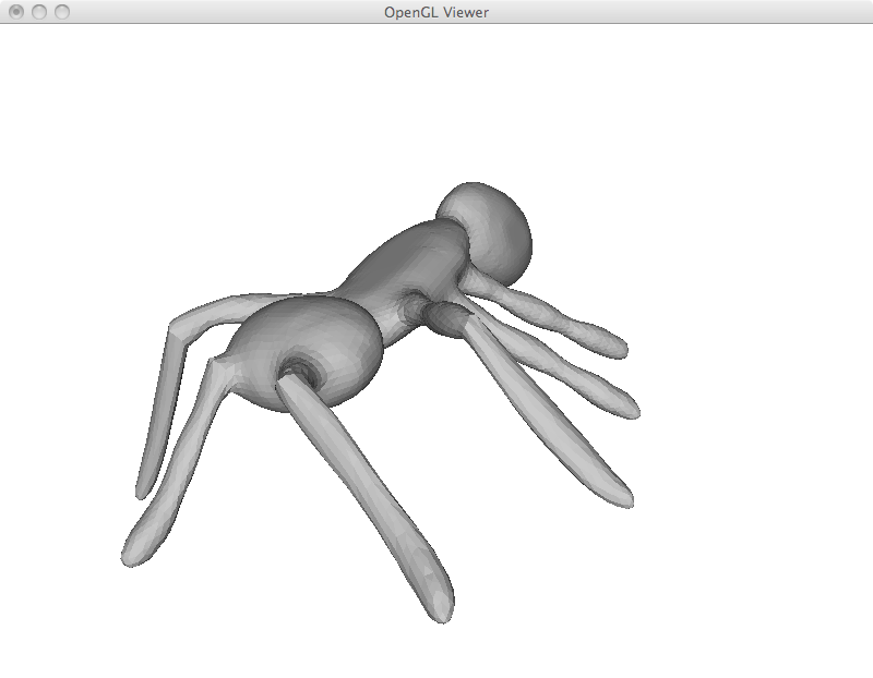
Region of interest
I implemented ROI control as described above. In the example below, it was used to move the limbs of the ant. As opposed to some of my first results, the user was not required to specify all anchor points, just the handle itself.
It was very important to include the Laplacian restriction on the handle. If we do not do it, this point works like a boundary condition of the Poisson equation. In the continuous setting, even though we are guaranteed to obtain a smooth interpolant inside the region where we are solving, the solution does not have to be smooth on top of the fixed point constraints. An example below shows the comparison of this two options. It seems like a minor change, but the results are completely different. Instead of least squares, a more formal way of solving this problem would be to look for a solution of the Bilaplacian equation. This equation would let you specify boundary hard-constraints on derivatives as well as positions.
Artwork
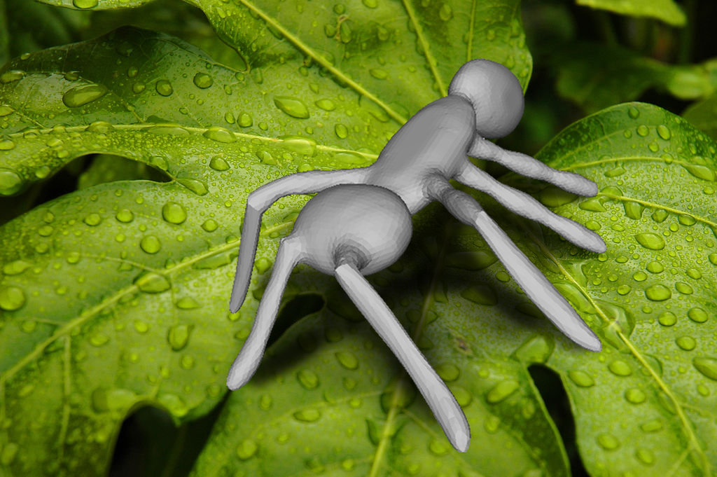
This final image was generated by deforming the ant's limbs so that their tips all lie in a common plane, i.e a virtual floor. This ant is rendered and composed with a background using an image manipulation program. An extra shadow was manually painted below the ant, perceptually it helps ground the ant on the leaf.
Acknowledgments
I am grateful to Tianqiang Liu, Jingwan Lu and Aleksey Boyko for interesting discussions and suggestions.
References
- Olga Sorkine, "Laplacian Mesh Processing", STAR report, EUROGRAPHICS 2005.
- CSparse library.