Sir Isaac Newton formulated the principles governing the the motion of two particles under the influence of their mutual gravitational attraction in his famous Principia in 1687. However, Newton was unable to solve the problem for three particles. Indeed, systems of three or more particles can only be solved numerically. Write a program to simulate the motion of N particles, mutually affected by gravitational forces, and animate the results. Such methods are widely used in cosmology, plasma physics, semiconductors, fluid dynamics and astrophysics.

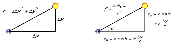
The physics. We review the equations governing the motion of the particles according to Newton's laws of motion and gravitation. Don't worry if your physics is a bit rusty; all of the necessary formulas are included below. We'll assume for now that the position (p_x, p_y) and velocity (v_x, v_y) of each particle is known. In order to model the dynamics of the system, we must know the net forces exerted on each particle.

• Pairwise force. Newton's law of universal gravitation asserts that the strength of the gravitational force between two particles is given by the product of their masses divided by the square of the distance between them, scaled by the gravitational constant G, which is 6.67 × 10^-11 N m² / kg². The pull of one particle towards another acts on the line between them. Since we are using Cartesian coordinates to represent the particles, it is convenient to break up the force into its x and y components (F_x, F_y) as illustrated below.
  
• Net force. The principle of superposition says that the net force acting on a particle in the x or y direction is the sum of the pairwise forces acting on that particle in that direction.

• Acceleration. Newton's second law of motion postulates that the accelerations in the x and y directions are given by: a_x = F_x / m, a_y = F_y / m.

The numerics.  We use the leapfrog finite difference approximation scheme to numerically integrate the above equations: this is the basis for most astrophysical simulations of gravitational systems. In the leapfrog scheme, we discretize time, and increment the time variable t in increments of the time quantum Δt. We maintain the position and velocity of each particle, but they are half a time step out of phase (which explains the name leapfrog). The steps below illustrate how to evolve the positions and velocities of the particles.

1. Calculate the net force acting on each particle at time t using Newton's law of gravitation and the principle of superposition.

2. For each particle:

   1. Calculate its acceleration (a_x, a_y) at time t using its force at time t and Newton's second law of motion.

   2. Calculate its velocity at time t + Δt / 2 by using its acceleration at time t and its velocity (v_x, v_y) at time t - Δt / 2. Assume that the acceleration remains constant in this interval, so that the updated velocity is:   v_x = v_x + Δt a_x,   v_y = v_y + Δt a_y.

   3. Calculate its position at time t + Δt by using its velocity at time t + Δt / 2 and its position at time t. Assume that the velocity remains constant in the interval from t to t + Δt, so that the resulting position is given by p_x = p_x + Δt v_x,   p_y = p_y + Δt v_y. Note that because of the leapfrog scheme, the constant velocity we are using is the one estimated at the middle of the interval rather than either of the endpoints.

3. Draw each particle.

Creating an animation. Draw each particle at its current position using Turtle graphics and repeat this process at each time step. By displaying this sequence of snapshots (or frames) in rapid succession, you will create the illusion of movement. After each time step (i) clear the screen using Turtle.spot("starfield.jpg"), (ii) write a loop to redraw all the bodies in their new positions using Turtle.fly and Turtle.spot, and (iii) let the turtle rest for a short while so that you can see what it drew using Turtle.pause(10). The parameter to the Turtle.pause command is measured in miliseconds: use it to controls the frame rate.

Input format. The input file is a text file that contains the information for a particular universe. The first value is an integer N which stores the number of particles. The second value is a real number R which represents the radius of the universe: assume all particles will have coordinates that remain between -R and R. Finally, there are N rows and each row contains 6 elements. The first two are the x and y coordinates of the initial position; the second two are the x and y coordinates of the initial velocity; the third is the mass; the last is a String that represents the name of an image file used to display the particle. As an example, the input file planets.txt contains actual data for our solar system in MKS units.

5
2.50e11
0.000e00 0.000e00 0.000e00 0.000e00 1.989e30 sun.gif
5.790e10 0.000e00 0.000e00 4.790e04 3.302e23 mercury.gif
1.082e11 0.000e00 0.000e00 3.500e04 4.869e24 venus.gif
1.496e11 0.000e00 0.000e00 2.980e04 5.974e24 earth.gif
2.279e11 0.000e00 0.000e00 2.410e04 6.419e23 mars.gif

Your program.   Write a program NBody.java that reads in the universe from standard input, simulates it using the leapfrom scheme described above, and animates it using Turtle graphics. Use StdIn.java to handle the data processing. Maintain several arrays to store the data. To make the computer simulation, write an infinite loop that repeatedly updates the position and velocity of the particles. Use Turtle graphics to create animation as described above. When plotting, be sure to scale the coordinates so that they stay within a 512-by-512 Turtle graphics window.

Optional finishing touch. For a finishing touch, play the theme to 2001 using the file 2001.mid. It's a one-liner using the method Turtle.grunt.

Extra credit. Submit a universe in our input format along with the necessary image files. If its behavior is sufficiently interesting, we'll award extra credit.

Challenge for the bored. There are limitless opportunities for additional excitement and discovery here. Try adding other features, such as merging bodies when they collide. Or, make the simulation three-dimensional by doing calculations for x, y, and z coordinates, then using the z coordinate to vary the sizes of the planets. Add a rocket ship that launches from one planet and has to land on another. Allow the rocket ship to exert force with consumption of fuel.