Human Computer Interface Technology
Digital Signal Processing for HCI
October 14, 2002
Perry R. Cook,
Princeton University
I. What's (a) DSP?
- DSP stands for Digital Signal Processing (or Processor)
- It's a branch of engineering mathematics which deals with the processing (filtering, detecting, etc.) of sampled data signals.
- If we make some assumptions, like the signals are sampled
uniformly in time, the systems we wish to study don't change
(much) with time, and the systems are linear (definition to
come), then the math gets very nice indeed.
- We care about DSP for HCI because we get lots of signals from our sensors and it's assumed that we want to do intelligent things with them in efficient ways. DSP gives us a set of tools that make certain things easier than the alternative: scratch our heads, try lots of hacks and heuristics, write lots of code, and fail.
II. Linear Time Invariant Systems
- A linear system is one that exhibits two properties:
- Homogeneity: If x -> y, then kx -> ky for any constant k
- Superposition: If x1 -> y1,
and x2 -> y2, then (x1+x2) ->
(y1+y2)
(NOTE: it's a convention that x is the input to a system and y is
the output)
- Examples of Linear Systems:
- Room acoustics is linear, because sounds simply add up,
and nothing changes except volume if you make the
sounds louder or softer.
- The outer and middle ear are essentially linear.
- Your stereo amplifier is linear (as linear as you can
afford), and any measure of distortion is a measure of
the non-linearity.
- One more property that's nice is Time Invariance,
which just basically means that the system behaves the
same independent of what time a signal is put into it:
- if x(n) -> y(n), then x(n+T) -> y(n+T), for any constant T
- OK, it's true that technically no system is time invariant,
because physical parameters change (you amplifier ages, you change
the volume and tone controls, etc.), but if the system is time
invariant over a suitable observation period, or only changes slightly,
or very slowly (relatively speaking), then we can still call it
linear for analysis purposes.
- Homogeneity: If x -> y, then kx -> ky for any constant k
- Superposition: If x1 -> y1, and x2 -> y2, then (x1+x2) -> (y1+y2)
(NOTE: it's a convention that x is the input to a system and y is the output)
- Room acoustics is linear, because sounds simply add up, and nothing changes except volume if you make the sounds louder or softer.
- The outer and middle ear are essentially linear.
- Your stereo amplifier is linear (as linear as you can afford), and any measure of distortion is a measure of the non-linearity.
- if x(n) -> y(n), then x(n+T) -> y(n+T), for any constant T
III. Convolution
- Linear, Time Invariant (LTI) systems can be dealt with
by using a mathematical operation called convolution:
y(n) = SUM[ x(n-T)h(T) ]
where h(T) is the "impulse response" of the system H. Another
way to think about the impulse response, and convolution, is
that h(T) is just the response y(n) for a special type of x(n).
called an impulse. That special impulse signal has value 1.0
at time zero, and value 0.0 all other times. This then means
that convolution is just the impulse responses of the system
to a train of weighted impulses (the individual samples of an
arbitrary x are viewed as just weighted impulses at different
times). Since the system is assumed to be LTI, we know that
the weighting (homogeneity) and delaying (time invariance) and
adding up (superposition) is legal.
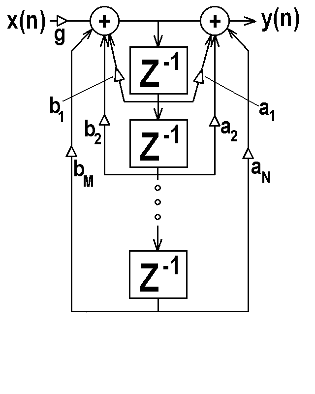
IV. Filters
- Digital Filters act linearly on a signal by forming
weighted sums of the signal, and also of past values of the
output of the filter:
y(n) = g[x(n) + a1 x(n-1) + a2 x(n-2) + ... + aN x(n-N)
+ b1 y(n-1) + b2 y(n-2) + ... + bM y(n-M)]
Linearity is obvious above, and if the coefficients
ai and bj are constant, then the filter is also time-
invariant. The figure below shows a generic linear
time invariant digital filter. The Z-1 blocks
represent a unit sample of delay.
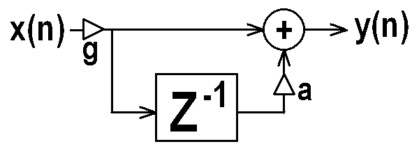
- A filter that only operates on the input signal,
but not past values of the output, is called a Finite
Impulse Response (FIR) filter. Such a filter would
only have non-zero ai coefficients in the above equation,
but all bj coefficients would be zero. We could also
note from our discussion on convolution
that the ai coefficients could be the hi sequence of an
impulse response of a LTI system. Thus, a digital FIR filter
can implement the convolution operation. The figure below
shows an FIR filter.

y(n) = g[x(n) + a1 x(n-1) + a2 x(n-2) + ... + aN x(n-N)
+ b1 y(n-1) + b2 y(n-2) + ... + bM y(n-M)]
Linearity is obvious above, and if the coefficients ai and bj are constant, then the filter is also time- invariant. The figure below shows a generic linear time invariant digital filter. The Z-1 blocks represent a unit sample of delay.
V. Special Simple Filters: One Zero
- The first order FIR filter is also called a "one zero"
filter:
y(n) = g (x(n) + a1 x(n-1))
- If we let g = 0.5 and a1 = 1.0, the one zero filter implements a two-point moving average, simply summing up the current sample with the one previous.
- If we let g = 1/T (the time interval between samples) and a1 = -1.0, then the two-point moving average approximates a differentiator
The frequency response of these two filters is shown here:

It's pretty easy to see that the moving average filter is a simple low-pass filter which blocks signals at 1/2 sampling rate entirely (that's the zero), and the differentiater is the complimentary high-pass filter. The signal processing block diagram of a one-zero filter is shown below.
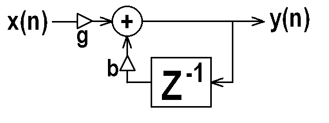
VI. Special Simple Filters: One Pole
- A filter that operates on past values of the output
signal (possibly in addition to past input samples)
is called an Infinite Impulse Response (IIR) filter.
Other names for this type of filter include "Recursive",
"Feedback", and "Auto-Regressive." The first order
IIR filter is also called a "one pole" filter:
y(n) = (g x(n)) + (b1 y(n-1))
- If we let g = 1.0 and b1 = 1.0, the one pole filter implements a "digital integrator", summing up all past input samples. This is not a very stable setting of the b coefficient, because feeding the filter a constant (DC) signal would result in the filter growing to infinity. Note also that any value of b which is greater than 1.0 in absolute value yields an unstable filter, which would grow to infinity for any input other than identically zero.
- Some useful common settings of the one-pole filter
are the
one-pole low-pass with 0 < b1 < 1.0, g = (1.0 - b1), and the
one-pole high-pass with -1.0 < b1 < 0, g = (1.0 - |b1|). - The signal processing block diagram of a one-pole filter
is shown below.
The frequency response of these two filters is shown here, with b1 = 0.9 on the left, and b1 = -0.9 on the right:

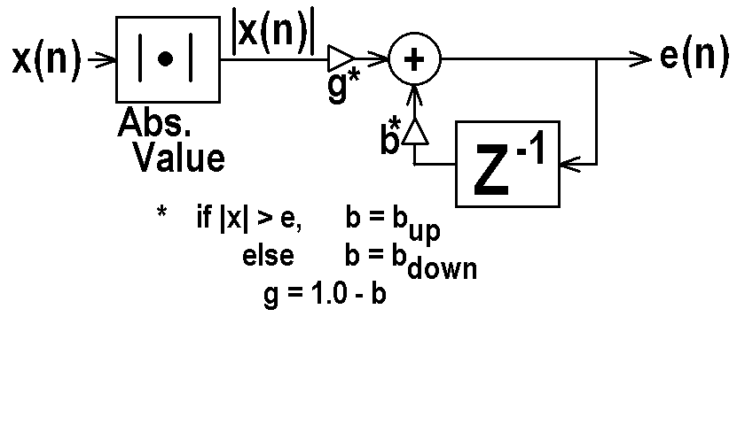
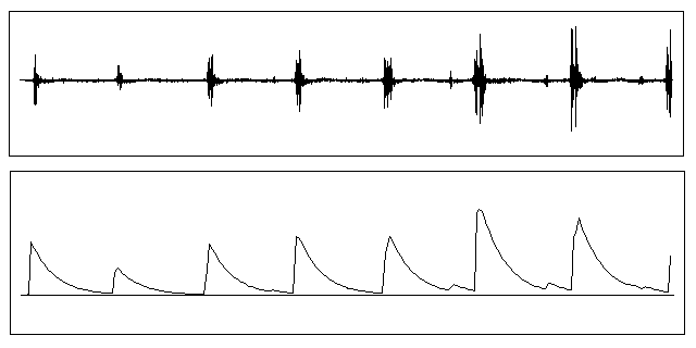
VII. Non-linear One Pole Application:
The Envelope Follower
VIII. Two Pole and Two Zero Filters
a/b_1 = 2 r cos(2 * PI * freq / SRATE)
a/b_2 = - r*r
where 0 < r < 1.0 is a resonance parameter
freq is the resonant or antiresonant frequency in Hz.
and SRATE is the sampling rate in Hz.
IX. Two Pole/Zero Applications: Tone detection and 60Hz. hum elimination
y(n) = x(n) - 2*0.9*cos(60.0*2PI/8000)*x(n-1) + 0.90*0.90*x(n-2)

X. The Fast Fourier Transform
* Permission to make digital or hard copies of part or all
of this work for personal or classroom use is granted with
or without fee provided that copies are not made or dis-
tributed for profit or commercial advantage and that copies
bear this notice and full citation on the first page. To copy
otherwise,to republish, to post on services, or to redistribute
to lists, requires specific permission and/or a fee.