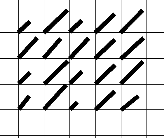
 We could then reconstruct the image by attempting smooth interpolation
as shown here.
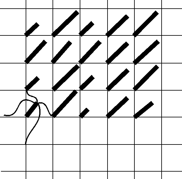
Motivation -- Much of computer graphics is driven by the quest for the perfect picture
Challenges
How are we going to address these?
Topics we'll cover
Sampling problem How do we best sample an analog (continuous) digitally (discretely)?
Reconstruction problem
Given that we have sampled, how do we best put the image back together?
Can we do so without losing any information?
Image enhancement Once we've sampled, there may be artifacts that we wish to filter out or there may be enhancements we wish to perform, how do we best do this?
When we sample an image, we do so by taking a set of samples
at points of a grid. We can think of the intensities at the samples
as being represented by spikes of appropriate heights as shown in the
picture For example,
a series of samples might generate the spikes
 We could then reconstruct the image by attempting smooth interpolation
as shown here.

Now, let's look at variations on a single image to illustrate out point.
We begin with the simple image
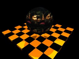 of a sphere ray traced over a checkerboard. We have texture mapped
an image from the course homepage onto the sphere. As it is, the image
appears very smooth.
We blow up a section of the image and notice the appearance of jaggies
along the edges of the checkerboard
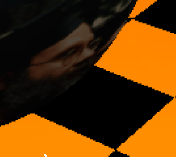 .
We wonder if we can smooth these edges to a nicer appearance.
Another example can be seen in the following images. We've
under-sampled our original image to make the pixels thicker.
We might ask if we can regenerate the original image.
 ,
,
 .
.
Next, we turn to filters that enhance images. For example, we might
want the image to appear blurred which we do with a low pass filter
that removes high frequencies which contain detail.
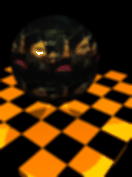 Or, we might want to sharpen the image in opposite fashion
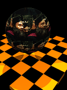 But we want to take care not to oversharpen it
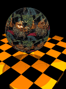
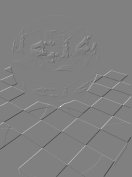
Next, we might want to locate high frequency components of an image,
which are places where significant change happens to locate e.g.
edges in the image. This converts our original image into a very different
representation
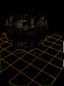 but by so doing, we allow ourselves to realize a number of
interesting effects
 .
.
Finally, we might wish to play with the colors in an image.
We might want to limit the number of colors,
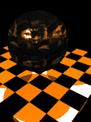 or produce a
grey scale image
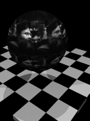 or even a grey scale image of few
colors (e.g. for printing in a newspaper) by a process called dithering.
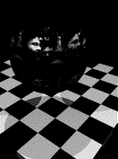
To address these issues, we will first study the representation of color and then study basic signal processing.
We have an image of intensity i(x,y) which is a real number between 0 and 1
at each location (x,y) but can only represent LEVELS different intensities.
Simplest form is to represent q(x,y) defined by
q(x,y) = trunc(LEVELS * i(x,y))
In this case, the error e(x,y) at (x,y)
would be q(x,y)/(LEVELS-1) - i(x,y). The total error in the image is
the square root of the sum of the squares of all e(x,y) values.
Such an approach can lead to contouring. Imagine an image where intensities change slowly, this will cause noticeable jumps. There are 2 solutions, non-uniform quantization and dithering.
This quantization worked on the assumption that all intensities
are equally likely and so all levels should be equal in size.
The assignment of intensities is as shown in the histogram

Suppose we knew otherwise. That is, if we had a histogram plotting
number of pixels per intensity, we might want to quantize to
respond to this histogram. How might we best do this?
For example, suppose we had the histogram
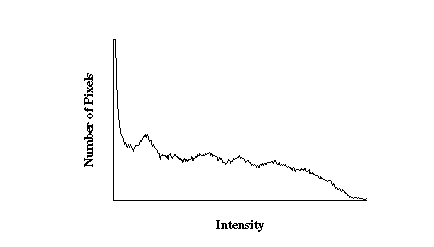 In this case, we'd prefer to assign levels somewhat like
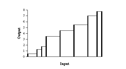
So, suppose that the intensity distribution of the image is p(i).
Then, the total quantization error is
 . What we've done is to sum the error over each
interval. We can optimize this by taking partial derivatives
and setting to 0 as
  .
When we solve the resulting equations, we determine the 2 necessary
conditions for optimality
  . The first of
these conditions
tells how to choose a value in a given interval (as its weighted mean).
The second says that given 2 adjacent means, their intervals should
be broken halfway between them. So, if we can find the means, we
know how to proceed.
The k-means algorithm due to Lloyd proposes a solution to this problem.
Often we have limited range of intensity with more than adequate spatial resolution and use a technique called halftoning. For example, in publishing we can turn a pixel on or off by drawing a black circle on a white backgroun. We want to use blocks of circles to simulate levels of gray. These techniques are known as pixel-grid patterning.
Sample patterns for 2x2 grids to represent 5 intensities might look like

Similarly for 3x3 grids, we might represent 10 intensities by
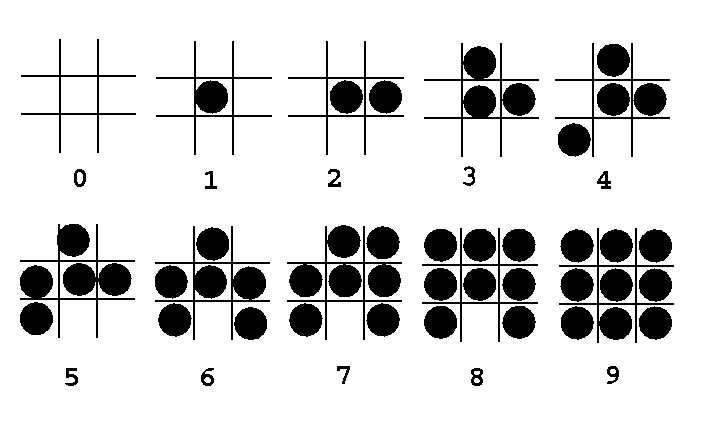
These choices have been made with some care.
The matrices
				|  8	3	7 |
B_2 =	|  3	1 |	B_3 =	|  5	1	2 |
	|  0	2 |		|  4	9	6 |
holds the choices for the 2x2 and 3x3 cases. We need to be careful to avoid some patterns. For example, the leftmost pattern is desirable to represent 2 when compared with the other 3 alternatives.

We can continue this process to generate higher order matrices where
B_n =	| 4B_{n/2} + 3*U_{n/2}		4B_{n/2} + 1*U_{n/2}	|
	| 4B_{n/2} +          		4B_{n/2} + 2*U_{n/2}	|
Note here that U_{n/2} is the n/2 by n/2 matrix of all 1's and
note that the coefficients of the U matrices repeat those of B_2.
These matrices are known as Bayer matrices. Halftoning in this fashion is often called applying a Bayer dither of size n.
The techniques described above are often called ordered dithering techniques for mapping of points in a scene to display pixels. Another method is random dithering by error diffusion. Here, the pixels are scanned in order and errors in realizing a pixel's intensity are distributed (ie diffused) to pixels to its right and below to keep the overall intensity of the image closer to the input intensity.
What we do here is choose values a,b,c, and d to represent the distribution to neighboring pixels. It is necessary that
a + b + c + d = 1For example, we might use the values (a,b,c,d)=(7/16,3/16,5/16,1/16) as shown in the figure
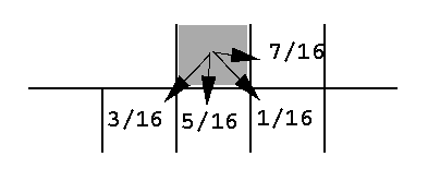
	for (i = 0 ; i < m ; i++ )
		for (j = 0 ; j < n ; j++ )	{
/* determine the intensity level Intensity[k] closest to the value M[i][j] */
			I[i][j] = Intensity{k];
			err = M[i][j] - I[i][j];
			M[i][j+1]   += a*err;
			M[i+1][j-1] += b*err;
			M[i+1][j]   += c*err;
			M[i+1][j+1] += d*err;
			}
The most popular error diffusion method is due to Floyd and Steinberg. In their method, a and c are set to 3/8, b is set to 0 and d is set to 1/4.
Now, we are ready to address the final piece of the puzzle.
As we said before, intensities are represented by the number
of electrons which excite the screen.
Once we've decided on relative intensities, we must decide how
many electrons will be fired.
Let us assume that intensity levels can be set to values between I_0 and I_1.
and ask for the n intensities to be shown in between.
Here we need to respond to the characteristics of the eye.
The eye sees intensities as relative values.
So, an algorithm that assigned values in linear fashion would
have more differentiation between low values than between high.
That is, the difference between intensities of .20 and .22 is
greater than the difference between intensities of .80 and .82.
To correct this, we work on ratios yielding.

Our final problem concerns the actual firing of electrons
and the display device. Typically, display devices have
response curves that follow the relation
 with respect to the electron-gun voltage (V).
Solving this for V yields
  .
Hence, we use the relation
  to determine the
number of electrons to fire to realize appropriately
intensity k.
Our images are bitmaps (or bytemaps) and so can be combined as such.
Typical operations
Examples
More sophisticated examples include chroma-keying, self-matting, ...
We need to introduce a few bits of mathematics to begin.
First, we say that a function is periodic of period T
if the function repeats itself outside of an interval of size T.
A simple periodic function is sin(x) which has period TWOPI.
We note that for all x, sin(x) equals sin(x+TWOPI).
There are other sine functions of different period. We will
change terminology and
say that the sine function sin(TWOPI f x) has frequency f
since it repeats itself f times more frequently than the
basic sine function.
A mathematical result dating back to the early 19th century states that almost any periodic function can be written as a (weighted) sum of sine and cosine waves (its so-called Fourier series). In our representation, we use the weights to represent contributions of different frequencies.
We might next ask what happens to non-periodic functions.
Of particular interest to us will be square pulses. For
example, we might want a function that has value 1 between -T and T
and value 0 elsewhere. Such a function is particularly poorly behaved
because of discontinuities at T and -T. In such cases, we
can approximate the function by a Fourier series of finite length
or realize it by a series of infinite length. For example, a square
pulse is the limit as n approaches infinity of the sum
 . As we plot the formula
for increasing values of n we notice that it converges
to the ideal square pulse.
In the limit, we replace the sum above by the integral
 where
where  and
and  . The F() values are the
coefficients of the sine and cosine terms. The function F is
called the spectrum of the function f.
We compute the spectrum via the integral
  .
This is called the Fourrier transform of f.
As we hinted above, we will be most interested in computing the Fourier transform of square pulses. Without filling in details here, we note that for a simple square pulse (f(x) = 1 if |x| < and 0 otherwise), the Fourier transform is defined by sinc(f) where the sinc() function is defined to be (sin(PI*x)/(PI*x)).
It is worthwhile to build up some intuition about Fourier transforms of particular functions. The Fourier transform of cos(wx) is 2 spikes, one at -w and one at w. The transform of sin(wx) is a positive spike at w and a negative spike at -w. The Fourier transform of a constant function is a single spike at the origin.
By a spike here, we mean a function which is zero everywhere but at the origin and infinite at the origin. It is really defined by its integral over the real line which is 1. The Fourier transform of a spike is a spike; that of a series of spikes is a series of spikes. This will be important when we get into sampling.
We close with some more terminology and a few observations. When we compute Fourier transforms we are able to distinguish components of different frequencies. A function with a spectrum containing no frequencies above some limit is said to be band limited. Typically, high frequencies in the spectrum of an image contribute to fine detail, sharp edges, ... Low frequency components represent large regions or objects. Referring back to the images at the start of this section, the edge detection was done by identifying high frequencies, blurring was done by removing high frequencies. Now we are ready to apply these ideas.
Filtering consists of modifying the spectrum of a function to enhance different frequencies. Examples
Low pass filter blurs, high pass filter sharpens. Filtering both ways separates the image into coarse and fine structure. The image is the sum of its two parts.
We can view filters via the following equation in the frequency domain
 where G() is chosen to select
those frequencies we wish to retain. Converting this equation to
the spatial domain yields the equation for what is called a convolution
 . A deep result that we will state
now is the Convolution Theorem which states that multiplying functions
in the frequency domain corresponds to convolving them in the spatial
domain. We can combine this insight with the Fourier transform
to implement the filtering operations we've described.
In the space domain, we sample by multiplying an image by a series of spikes as we saw above. In so doing, we throw away information everywhere except at the sample points.
In the frequency domain, this corresponds to convolving the spectrum of the image with a series of spikes (spectrum of the sampling spikes). This convolution then creates multiple copies of the image. We now use a low-pass filter to reconstruct the image.
The sampling theorem of Shannon says that we can do so exactly if the original signal has no frequencies above half the sampling frequency.