

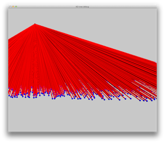
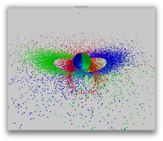
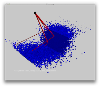
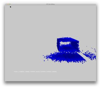
A point light source shoots light in all directions, with equal probability. We show the results of photon emission from a point light source in two scenes: one with a single light source and the other with 3 light sources. The scenes consist of a sphere on a box.
Note that the light source emits photons in all directions. We only show photons that hit the scene. Each small sphere represents a single photon. A tiny line on the sphere represents the incident direction. Photon colors are consistent with the power they hold.
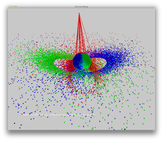
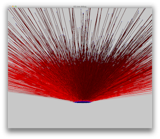
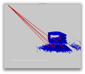
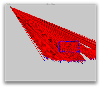
Scene 1: single blue point light. Rays are used to illustrate the photon path. Images show (from left to right) no rays, some rays and all rays.
|
|
|
|
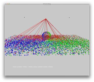
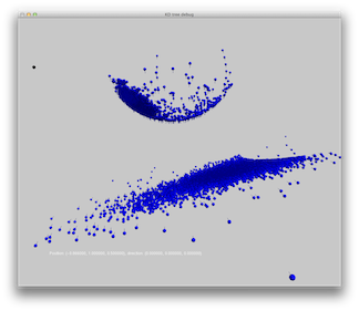
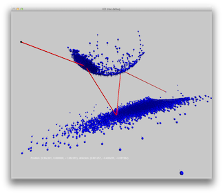
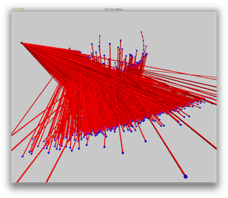
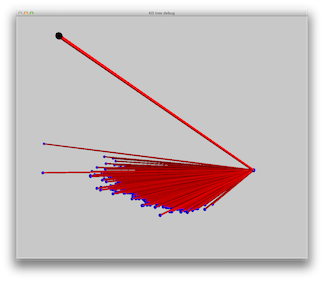
Scene 2: three point lights - red, green and blue.

|
|

|
For an area light source, we need to shoot photons from a random location on the surface of the light, towards a random diffuse direction. In this project we implement circular area lights only, but this can be easily extended to arbitrary shapes. The sampling is done using rejection sampling for location, and using a simple transformation from 2 uniform random variables for the direction.
Scene 3: two spheres on a box. White area light coming from above.
|
|

|
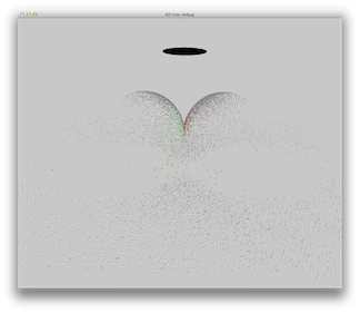
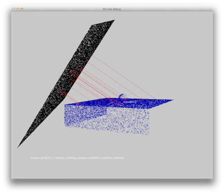
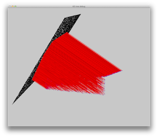
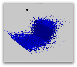
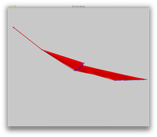
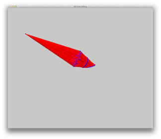
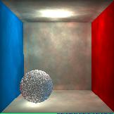
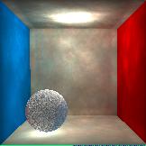
A directional light source aims to simulate a light source very far away (e.g. the sun). We simulate such behavior by shooting rays from an area light which is completely outside the scene. All rays are shot in the same direction.
Scene 4: A sphere on a box, one blue directional light. Area used as emission points is marked in black.

|
|
|
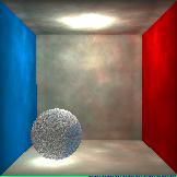
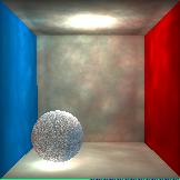
Scene 5: A sphere on a box, three directional lights - red, green and blue.

|

|

|
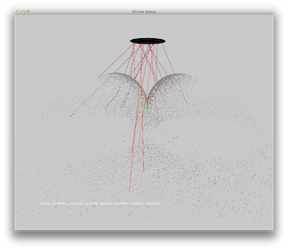
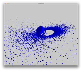
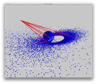
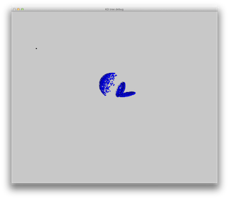
For a spotlight source, we need to shoot photons in an amount which is proportional to the cosine of the angle between the light direction and the shooting direction, raised to the power of n, where n the drop-off rate.
Scene 6: A sphere on a box, single blue spot light. Notice that rays that bounce off the sphere are also shown. Reflection and refraction will be discussed in later sections. Also notice that no cut-off angle was implemented, since did not seem to influence rendering results too much. A cut-off angle can be easily added.
|
|

|
Scene 7: A sphere on a box, three RGB spot lights.
|
|

|
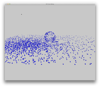
We show a scene with a spotlight pointing downwards. The light hits a diffuse box, which scatters the photons to all directions. The photons are absorbed in a large box above the spot light (which is set to absorb all light).
Scene 8: A large absorbing box above a diffuse box. A blue spotlight is directed towards the diffuse box.

|

|
|
Scene 9: A box on a box. The materials are almost completely specular. A single spot light is used.
|
|

|
Scene 10: A sphere above a box. The materials are almost completely specular. A single spot light is used.
|
|
|
When dealing with transparent materials with different indices of refraction, the photons obey Snell's law. We use 2 test scenes. Each has a specular box as a base. Above the box there is a hovering transparent box in scene 11 and a hovering sphere in scene 12. A blue spot light is illuminating both scenes.
Scene 11: A transparent box above a specular box.
|
|
|
Scene 12: A transparent sphere above a specular box.

|

|

|
Up until now we have used the exact reflection / refraction angle for outgoing photons. This causes sharp unnatural edges in rendered images. We now build upon the previous implementation, and add importance sampling to the direction of the outgoing photon. When doing so, a single outgoing direction becomes a lobe of possible outgoing directions. We show results before and after adding the lobe sampling.
Reflection example. Left: only one outgoing angle. Middle: a lobe of outgoing angles, n = 1000. Right: A lobe of outgoing angles, n = 100.

|

|
|
Refraction example. We shoot rays through a transparent sphere. Left: only one outgoing angle. Middle: a lobe of outgoing angles, n = 1000. Right: A lobe of outgoing angles, n = 100.

|
|

|
We implement two photon maps, one for all ray paths and one only for LS+D paths. This separation is done because we need a lot more photons to get high quality caustic effects. By separating the two maps, we can use a small number of photons for the global map and many photons for the caustic map. We show the two maps for the same scene: a glass sphere above a diffuse box, with a single blue point light.
Top row: caustic photon map. Bottom row: global photon map.
|
|
|

|
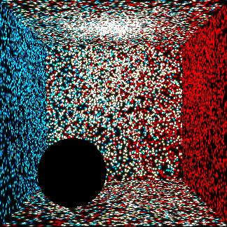
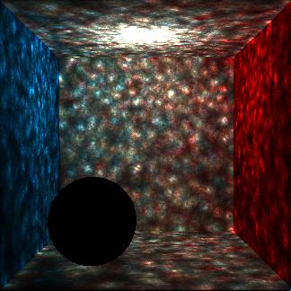
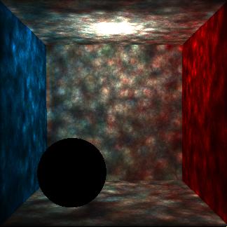
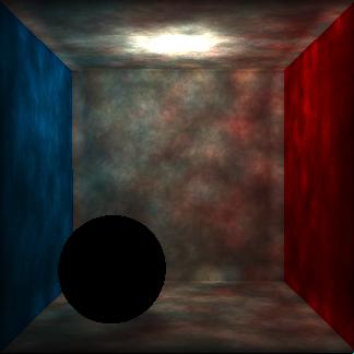
We shall start by directly rendering the photon map. We use the scene kindly provided by Abu which has colored diffuse walls, a transparent sphere and a point light. Here we demonstrate how the amount of photons used for radiance estimate affect the result. Results use 1, 5, 10, 20, 60 and 100 photons for the estimate, respectively. Notice the color bleeding on the walls. Only the global photon map is shown.
|

|
|
|
|

|
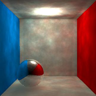
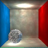
We present here several Cornell box variants, to showcase several lighting phenomena. We show a box with diffuse walls, a single point light and a sphere in the middle of the box. Several versions of the sphere are shown: diffuse, specular and transparent.
From left to right: diffuse sphere, specular sphere and transparent sphere. Notice the color bleeding on the walls and on the diffuse sphere. Also notice the specular highlights on the specular sphere and the caustics due to the transparent sphere. The specular sphere has a black area in the middle, since the box is not closed (there is no back wall) so blackness is reflected.

|
|
|
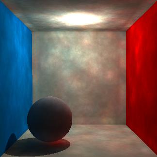
While theoretically the global photon map should contain data about shading, it is sometimes the case that the shades are obscured due to other details. For example, in all the examples presented until now, a hint of shade (cast by the sphere) is visible, but this shade is overwhelmed by the amount of light reflected off the diffuse walls. In order to get clearer shades, we can trace rays towards the lights, as demonstrated below.
Left: no shade enhancement, right: shade enhanced by tracing rays toward lights and checking for occludes.
|
|
|
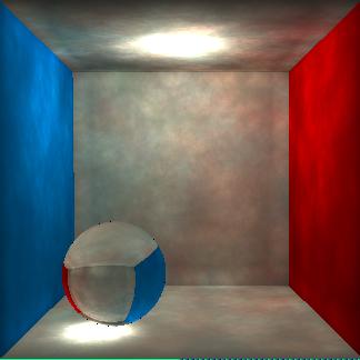
We can shoot multiple rays for each pixel, and take the mean of all results as the pixel value. We demonstrate the affect of multiple samples using a sphere which is half-transparent. Since we shoot rays in a probabilistic way, when only 1 sample is used per pixel, we get a noisy result for the sphere - some pixels act as transparent while others as opaque. When using multiple rays this behavior averages out, as needed.
From left to right, top to bottom: 1, 2, 3, 4, 5, 6, 7, 8 and 9 samples per pixel.
|

|

|

|
|
|
|
|

|
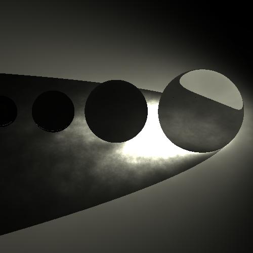
Inspired by Abu, I wanted to create a planetary system kind of feeling. Not sure I got the exact effect, but still I think the look is nice...
|