Photon Mapping

Nora Coler

Overview

For this assignment, I implemented photon mapping as described in the Jensen paper.

Phase 1: Photon Tracing

Photon emission:

I emitted photons from the different light sources based on a uniform distribution. The power of each photon was divided by the total number of photons emitted from that light. The point light photons were sampled from a sphere. The spot light photons were sample from a cone based on the spot light parameters. The directional and area lights were sampled from a disk. The directional light's radius was based from the diagonal of the bounding box of the scene.

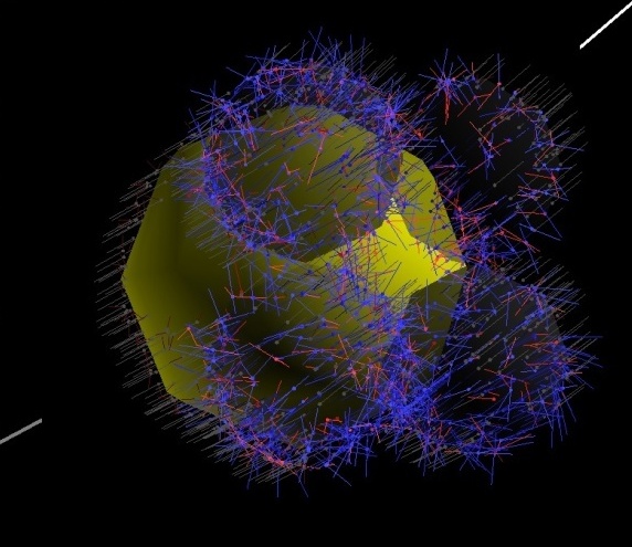
Photon scattering: 

Photons were stored in the following structure so that they could be easily drawn for debugging.

struct Photon

{

R3Point position;

R3Vector direction;

R3Vector newDirection;

RNRgb power;

int bounces;

BounceType inType;

BounceType outType;

}

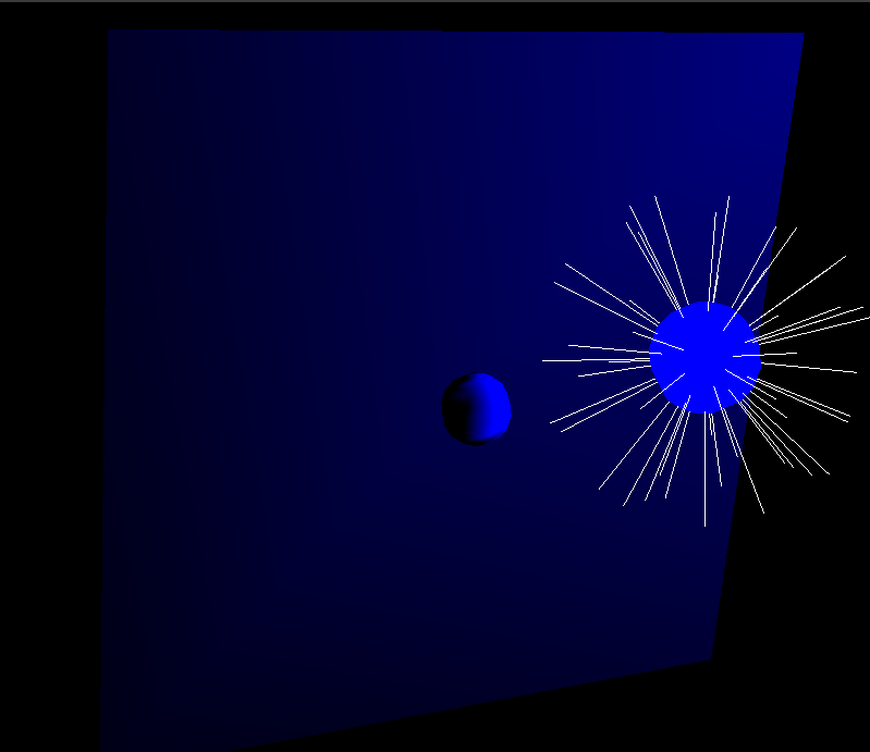
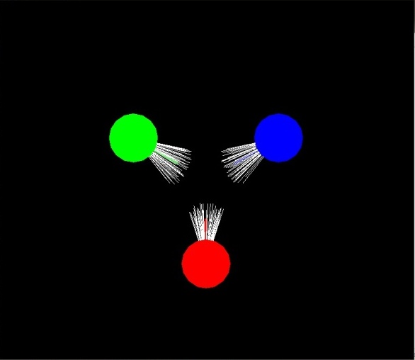
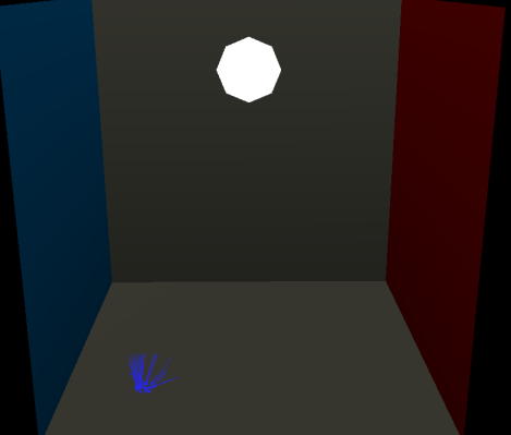
Whenever a photon hits a diffuse surface it was stored. Then it was sent on using Russian Roulette based on the probability of the diffuse, specular and transmission colors. The probability was calculated based on Jensen's notes. The resulting powers were also adjusted according to Jensen's formulas. The random number to determine which path to take was chosen from the interval 0 to max(1, probability Diffuse + probability Specular + probability Transmission). This way non realistic materials could be taken into account. The diffuse directions were sampled from a uniform hemisphere. The specular direction was sampled from an area determined by the specular coefficient around the perfect reflection direction. Transmitted rays were calculated based on Snell's law. When sending off the new photon, it's position had to be adjusted by an epsilon value in the direction that it would travel so that it would not intersect with the surface that it just landed on. After 5 bounces the photon was stopped. The pictures below show photons in different scenes. The lighter the photon, the more bounces it has taken. The long lines from each point are where the photon has come from. The short lines are where the photon is going. Red means it was generated from diffuse distribution, green means specular distribution, and blue is the refraction. Gray means the ray came from the light source.

Multiple photon maps:

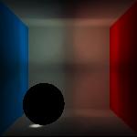
I implemented both a global photon map and a caustic photon map. For the caustic photon map, the photons could only be directed in the specular direction or refracted. The direction was still chosen based on the same probabilities of the global photon map. Once the photon hit a diffuse surface, it was stored and terminated. Above are the pictures of the global photon map. Below is a picture of the caustic photon map.

Phase 2: Rendering

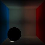
Camera ray tracing: 

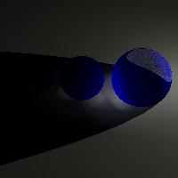
For each pixel, I traced a ray into the scene. Then, I traced them through the surface interactions using the same method as the photons. The probabilities of how it was scattered were determined by averaging the components of the diffuse, specular, and transmission colors respectively. The color of the below picture has the same legend as tracing the photons.

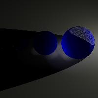
Radiance estimation:

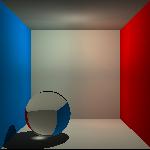
The kdTree for the global photon map and the caustic photon map where used to compute the closest photons. Once the kdTree return the closested N photons, the radiance was computed by the sum over the power times the BRDF divided by the area of that the photons were gathered from. The below pictures were created by using cone filtering as well. The max photons was set to 2000 for global and 1000 for caustic. The max distance was set to .5 for global and .05 for caustic. To create the Cornell pictures, 2000 photons were used with 1 ray per pixel. To create the glass spheres, 4000 photons were used with 4 rays per pixel.

Pixel integration:

I also added a variable so that you can change how many rays are sent out per pixel. The values returned from each ray were averaged together to get the final pixel color. The default is 4 (2x2).

Additional Options:

Filtering:

I implemented cone filtering to weight the photons during the radiance estimate.

More Images

Final Cornell Image: Started with 5000 photons and 16 rays per pixel

Snowman: Started with 7000 photons and 4 rays per pixel

Violin: Started with 5000 photons and 16 rays per pixel