Photon Mapping
COS 526 Programming Assignment 1
Maciej Halber
Introduction
Photon Mapping is a global illumination rendering algorithm, that aims at reducing rendering time compared to techniques like Path Tracing, via introducing a preprocessing step of photon tracing. The photon tracing stage shoots photons from every light source in the scene and traces their interactions within it. Photons are stored on diffuse surfaces, reflected from specular surfaces and transmitted through transparent ones. As photon goes through the scene we store its position and power at the point of photon ray-scene intersections. This creates photon map (hence algorithm name), which is then used in the subsequent rendering stage, which is essentially a path tracer[1] that takes an advantage of the pre-computed photon map.
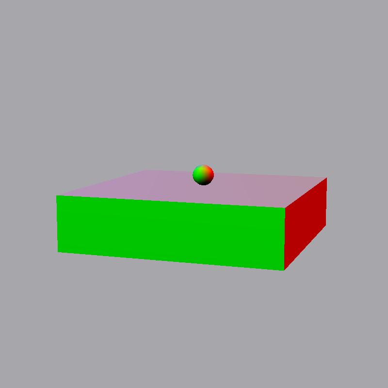
Provided implementation takes in various arguments which control the way image is produced. All these settings are stored in the RenderSettings structure in render.h. These parameters are pretty self explanatory and we will refer to them in subsequent sections of this report on their influence on particular aspects.
Mappings
Being able to generate random positions on 2-manifold is extremely important for a software like photon mapping renderer - at each surface intersection we need to randomly generate an outgoing ray. Jensen[1] provides a section on mapping an unit square [0,1) to a range of 2-manifolds. In this implementation we have created function that take points distributed in unit square to various different to manifolds (fig.1). Implemented mappings include plane-to-plane, plane-to-disk, plane-to-sphere, plane-to-hemisphere and plane-to-phong lobe, and are used when generating the random rays throughout both stages of the algorithm (photon tracing and rendering).
Photon Tracing
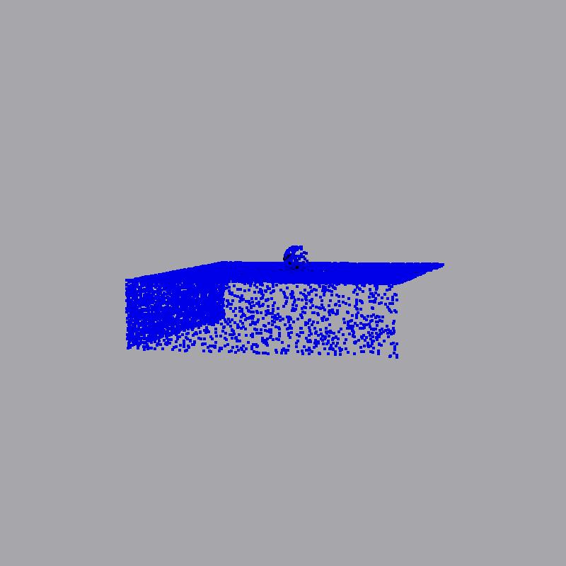
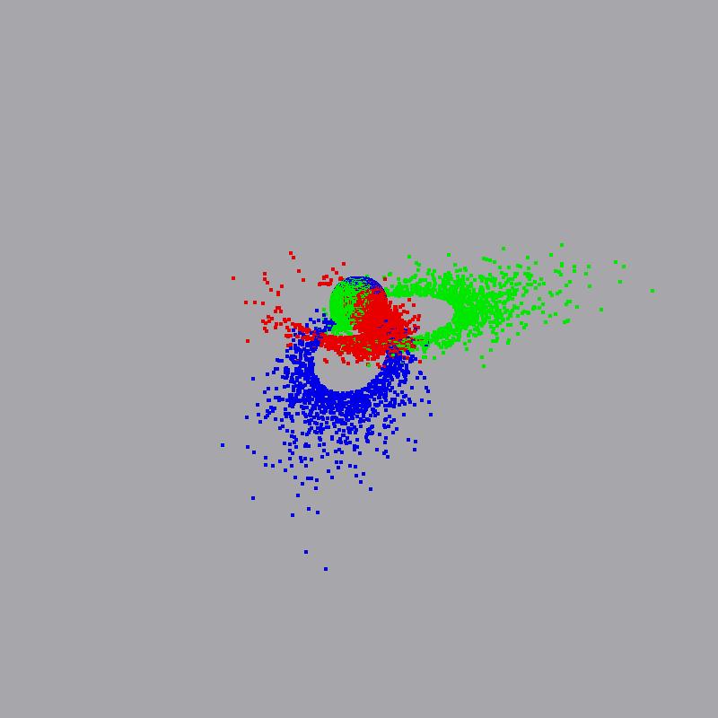
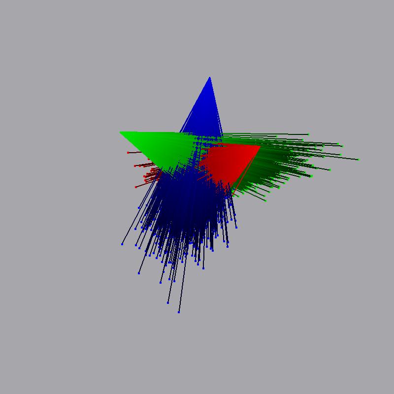
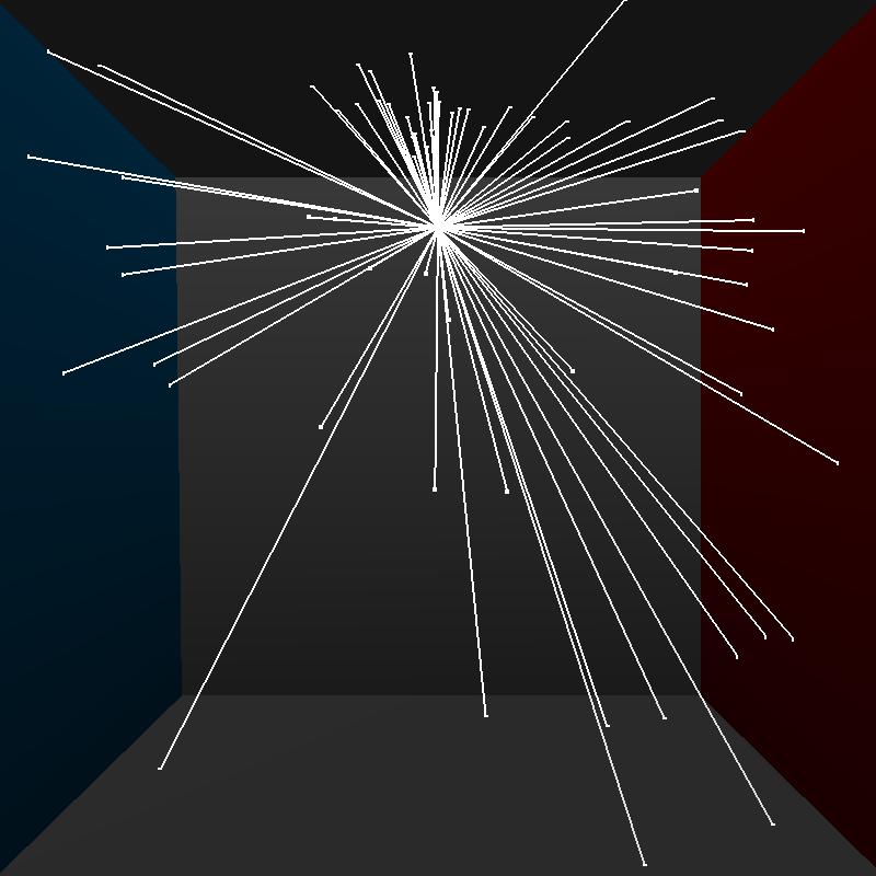
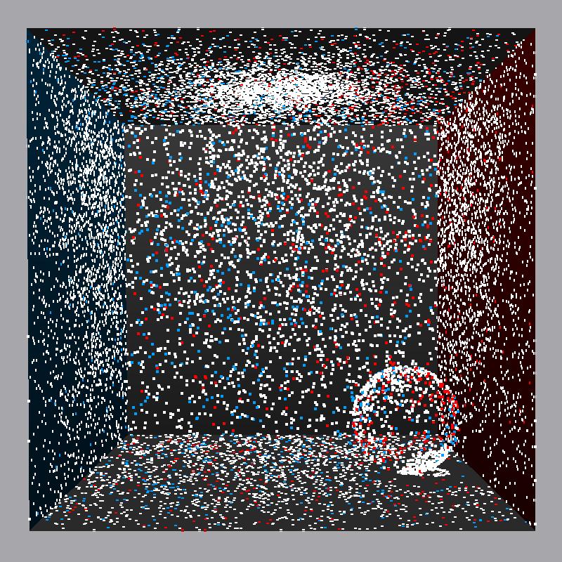
A central part of the implemented system is to emit photons from each light and trace them through the scene. To aid understating of the algorithm and as a debugging tool, it was crucial to implement viewer features that help us investigate the behavior of our photon tracer. Here we will illustrate the features of implemented renderer - emission from various light sources, the traversal through various media, as well as storage of photons. Implementation wise, the program provides arguments n_photons and n_caustic_photons to control how much photons are shot to the scene for both photon maps (discussed below). The number of photons shot is proportional to the intensity of the light source, while the photon power is kept constant.
Photon Emission
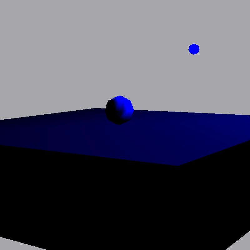
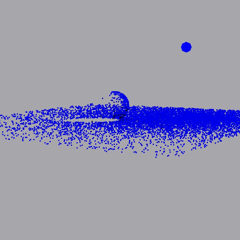
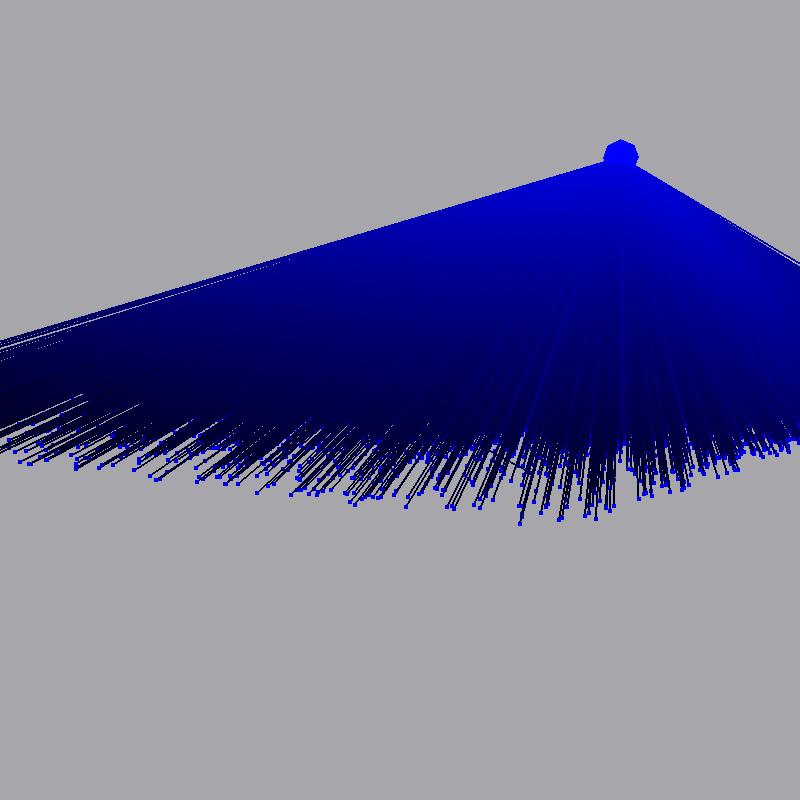
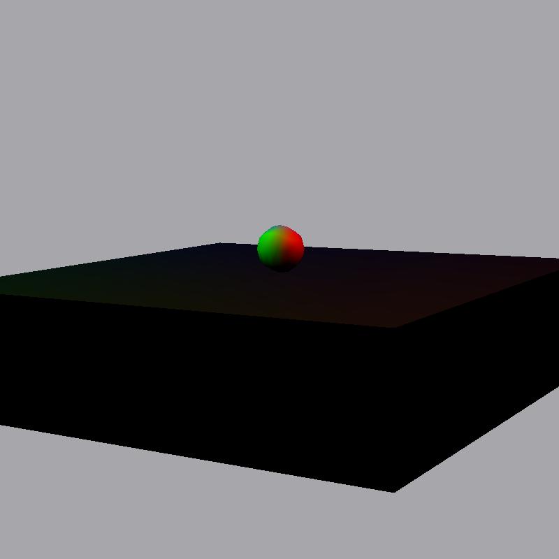
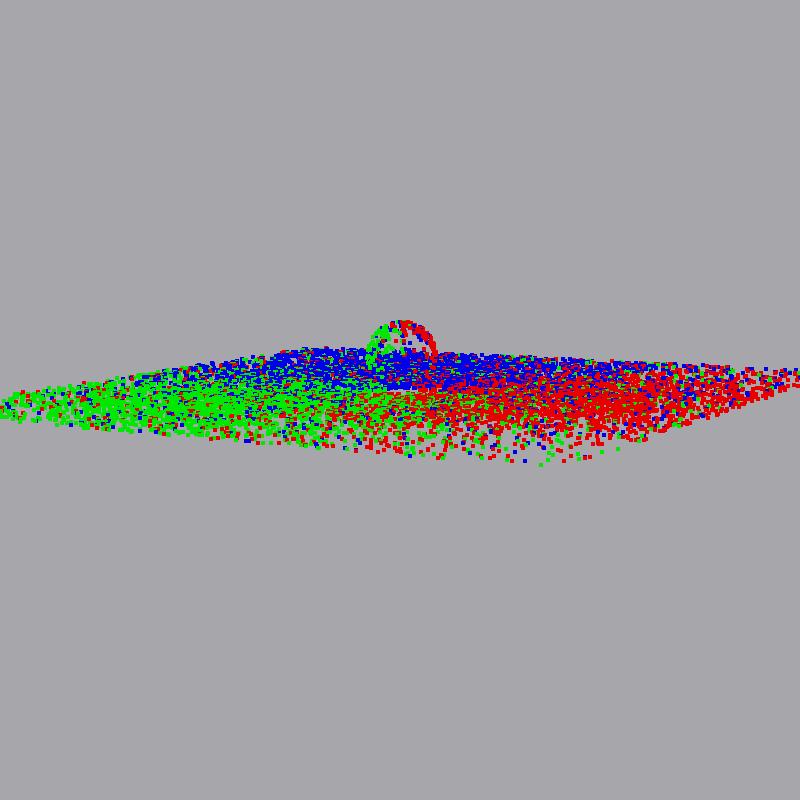
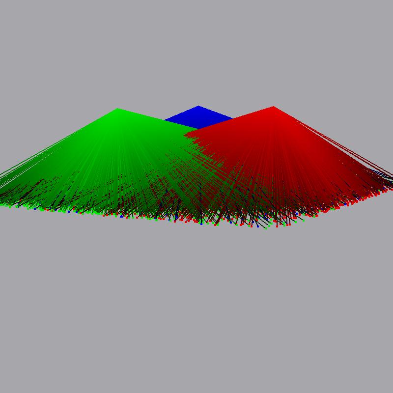
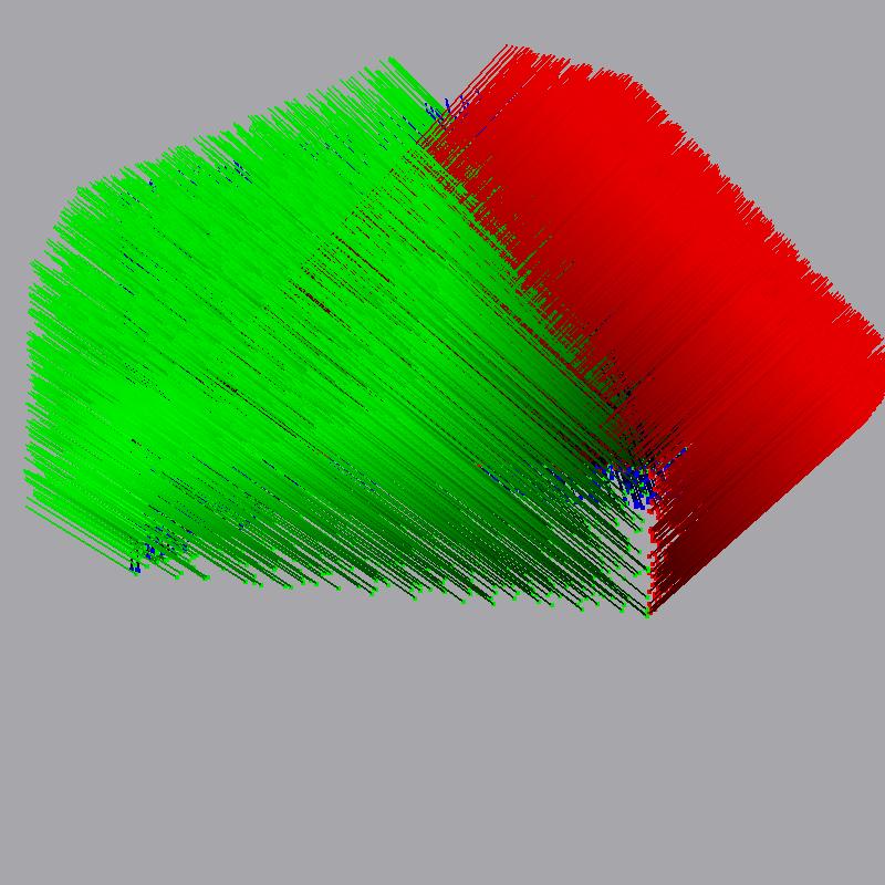
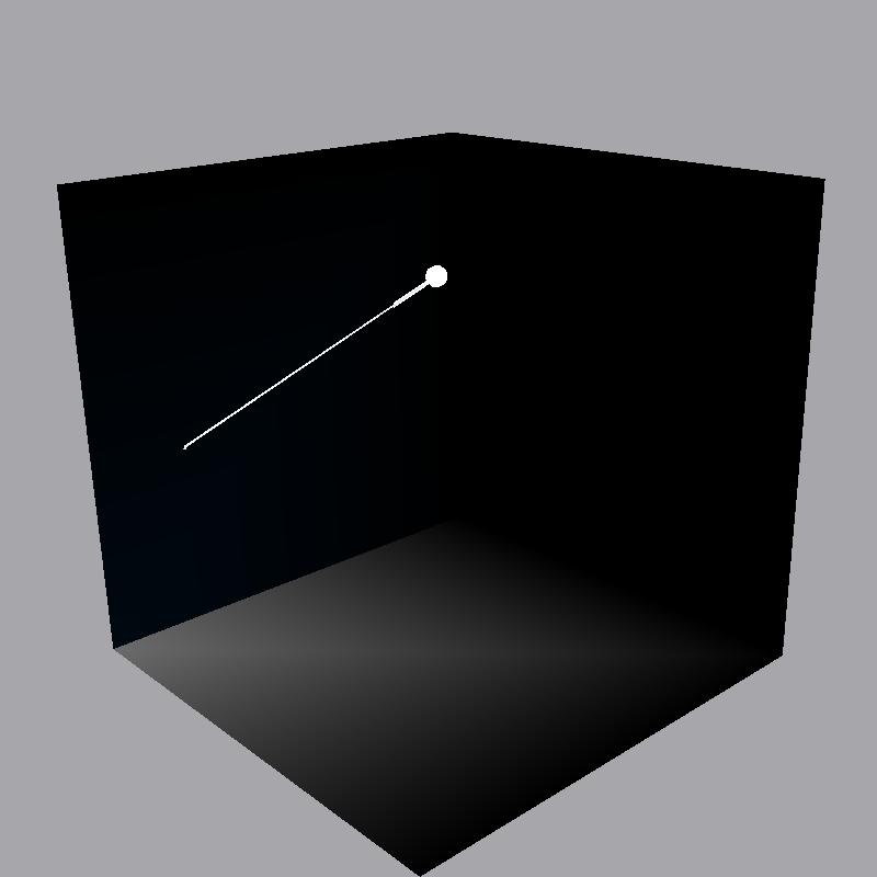
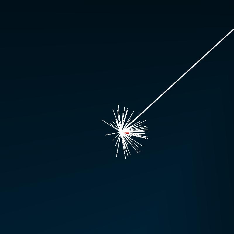
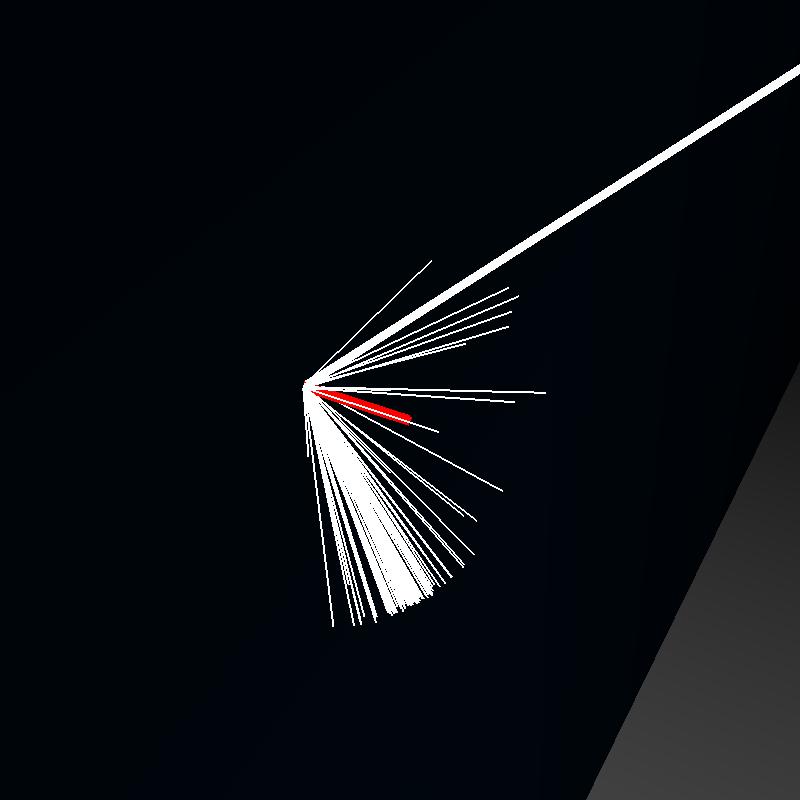
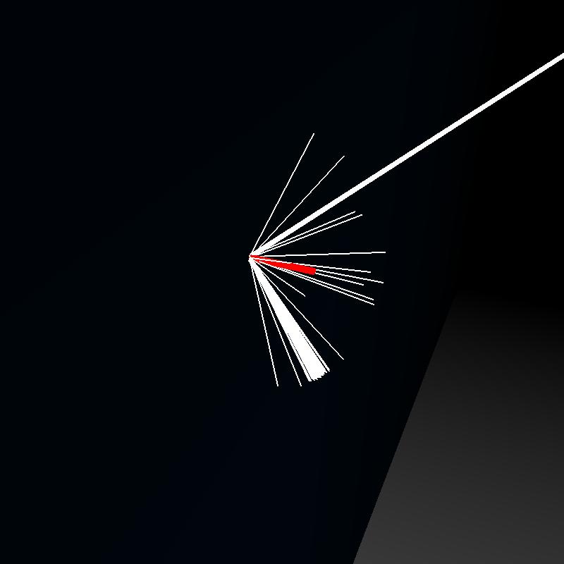
Point Lights
Here we show two scenes containing point lights, alongside with visualization of photon maps and the rays. Notice that these images only show the first intersection with the surface and no subsequent bounces for presentation clarity. Viewer allows for control of regulating what number of bounces is shown, via "+" and "-" keys. Also note that point lights shoot rays in spherical direction, however through rejection sampling we have retained only the rays that intersect the scene.
Directional Lights
Directional lights are lights that conceptually simulate light source like sun - that is they are shot from large area outside the scene and all rays are parallel.
Spot Lights
Spotlights can be thought of as alight source similar to a flash-light. They are defined with a point p, direction dand a drop-off rate k. That is we shoot rays from p in approximate direction d, conditioned on k. Large k will bring our spotlight to behave more like a laser.
Area Lights
Area lights are the only physically plausible light sources in our system, in this implementation they are shaped as a disk. We sample random position on the disk and then for each of these positions we create random direction on a hemisphere oriented along the area light normal.
Photon scattering
Importance sampling
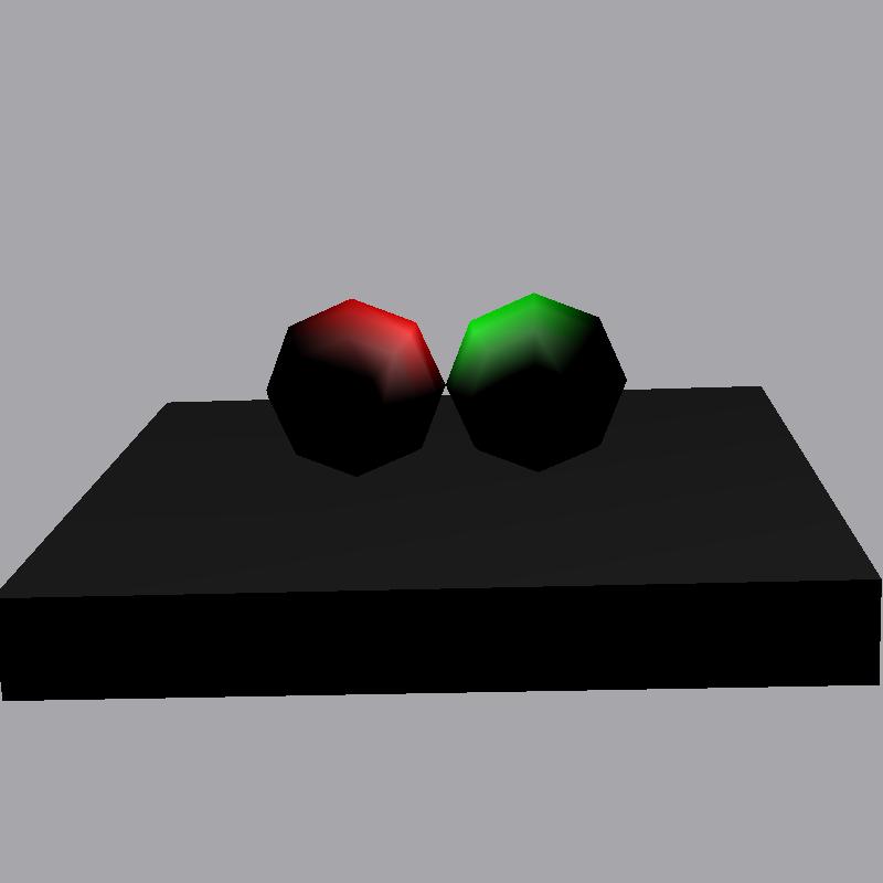
Different materials will reflect incoming photons in a different way - diffuse surfaces will reflect incoming photon in the random direction on a hemisphere, while specular materials will have higher probability to reflect incoming ray in direction similar to the direction of perfect specular reflection. Here we present the interaction a photons will undertake while hitting a various kinds of surfaces.
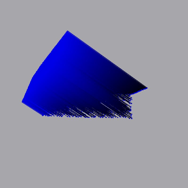
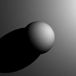
Refraction
Below we show a rays traversing through a glass sphere, to illustrate the ray bending when coming through a medium with different IOR. For presentation clarity we are providing the images showing various number of photons being shot.
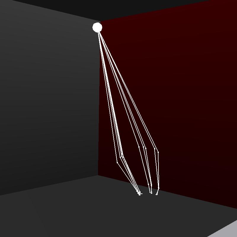
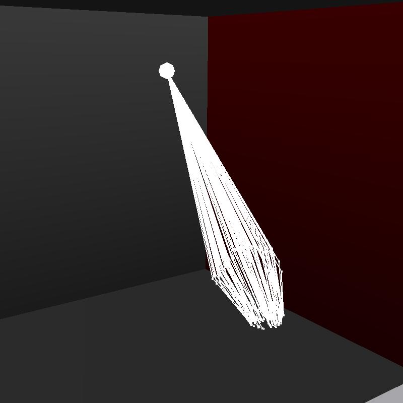
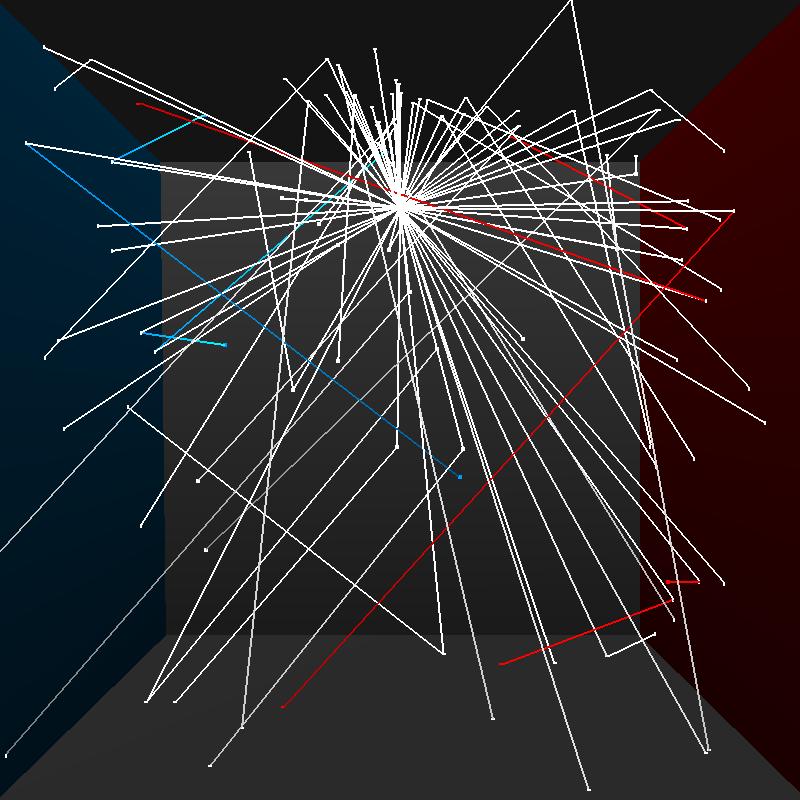
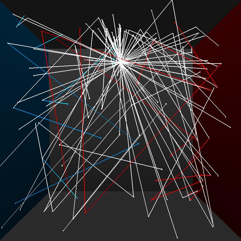
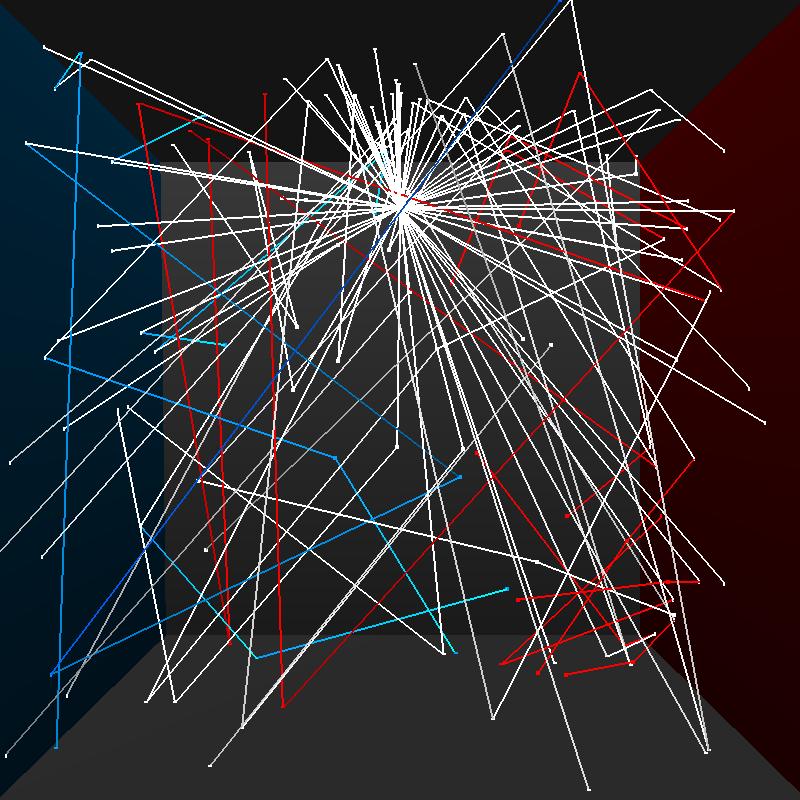
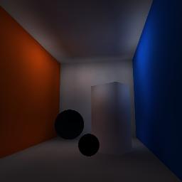
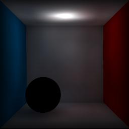
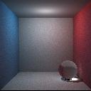
Cornell box bounces
Here we present visualization of photons bouncing around in a cornell box scene provided with this assignment. For clarity of visualization we have only shot 100 photons into the scene
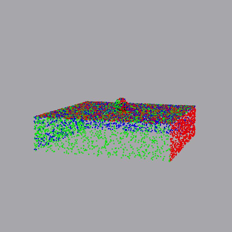
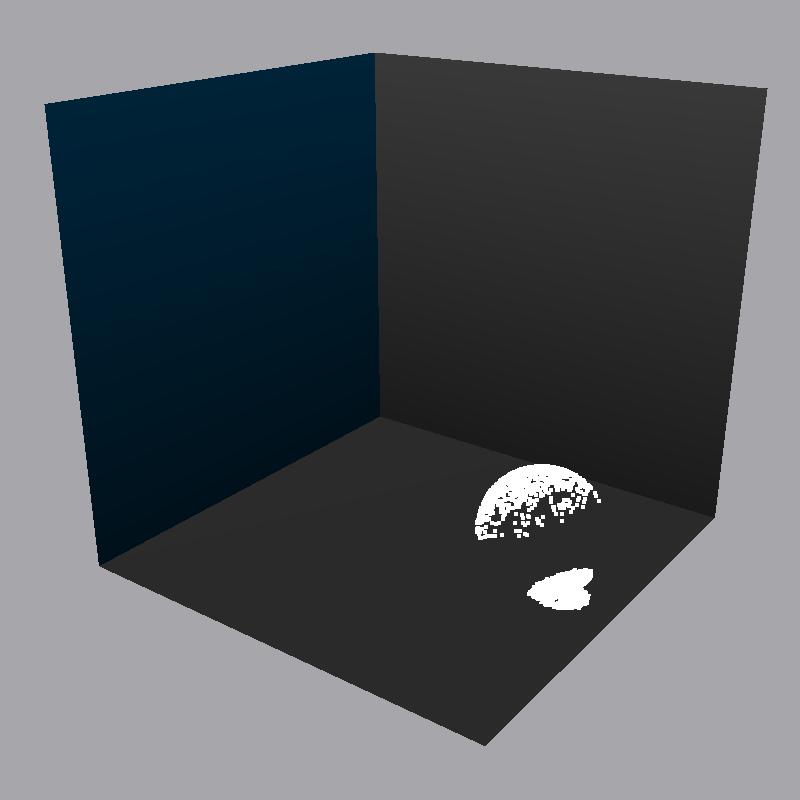
Multiple photon maps
Here we present two photon maps stored by my program - the global photon map, storing interactions with all surfaces(all paths), and a caustic photon map, which stores LS+D paths. Note that for visualization purposes we store photons when they interact with non-diffuse surfaces. These are not used while rendering. Purpose of using the two maps is to improve the appearance of caustic effects - lights taken by photons that create these effects are usually quite complex and the probability that we will trace them using path tracing or even global map photon tracing is low. Thus we introduce second map to specifically create these caustic effects.
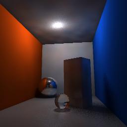
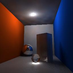
Shadows
A basic part missing from the initial ray tracer we have been provided with as part of this assignment, was shadow computation for direct illumination (clearly present in Jensen01). We have implemented the shadow computation for all light sources - the most interesting light source is of course the Area Light, since it produces soft shadows. The amount of noise is dependent on the number of rays we shoot through a pixel -- the higher the number, the softer, less noisy shadow becomes. All images in first row below were rendered using 4 samples per pixel.


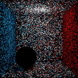
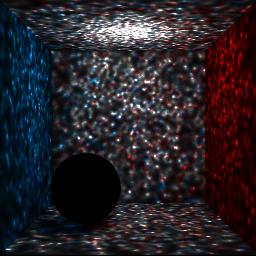
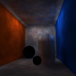
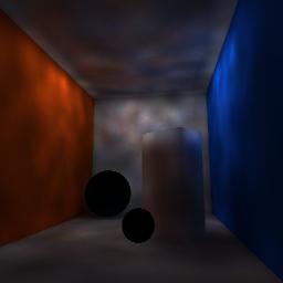
Radiance Estimation
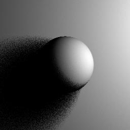
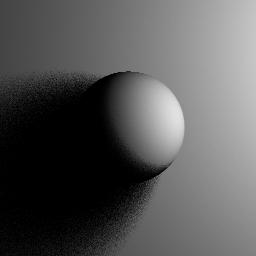
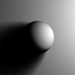
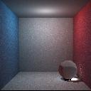
During the photon tracing step of the algorithm we have created a photon maps, which we have shown in Visualization section. We can also render the photon maps, by shooting a ray through a scene and querying the kd-tree for nearby points, and then estimating radiance coming from given position. This procedure's result will of course depend on parameter, namely the number of nearby photon we ask to find around position x. Below images show radiance estimate for two scenes, cornell box provided with this assignment and custom cornell box - like scene we have created in Blender and exported to .scn format using script kindly provided by Nikhilesh Sigatapu. In all images we have shot 9192 photons and varied number of nearby photons used for radiance estimation. n_nearby_photons is one of the parameters to my program, stored in RenderSettings structure. It is interesting to see, that the indirect illumination smoothens nicely with the increase of the number of photons used in estimation, however we are also making shadows less apparent in the same process. This was one of the motivations to implement shadows calculations shown in previous section.


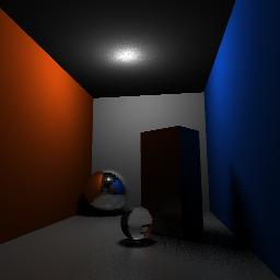
Rendering
Rendering part is done as distributed ray tracer. As such we can ask the renderer to render images of different types. In provided implementation we allow user to query for various types of render. These include direct illumination only, caustics, approximate rendering, approximate rendering without caustics, full rendering.
The full rendering is full photon mapping algorithm where we perform path tracing, that is when we shoot a ray from camera and we hit diffuse surface we create n_glob_illum_samples secondary rays in directions of diffuse surfaces and gather estimate the radiance from each of those. As such this technique requires many rays to lower the variance in our estimate and takes a long time to compute. Due to that our results are either small resolution or bit noisy
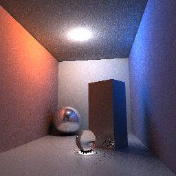
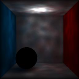
To account for that we have approximate rendering render types. These are similar to full rendering, however when ray from camera hits diffuse surface the radiance estimate is performed at intersection point, however it ignores the photons from direct illumination (i.e. it takes only photons from secondary bounces into account), to prevent double counting radiance estimation and direct illumination. This results in less correct images, but much improved render times. The approximate rendering without caustics render type is self-explanatory - we ignore the caustic map when rendering. As seen below this technique still can give us quite pleasant, and most importantly noise-less results.
Cone Filtering
We have implemented cone filter to smooth the results of radiance estimation and reduce false bleeding Especially notice the reduction in artifacts around the edges and corners of the box. User is able to provide the program with argument cone_filter, which needs to be value larger or equal to 1. All images in this report have been using cone filtering with k = 1.2.
PerPixel Sampling
As seen with the area shadows, system allows user to proviede n_per_pixel_samples argument, which will determine number of rays shot through a pixel using stratified sampling. More samples lead to better full rendering results, better area shadows and antialiasing.
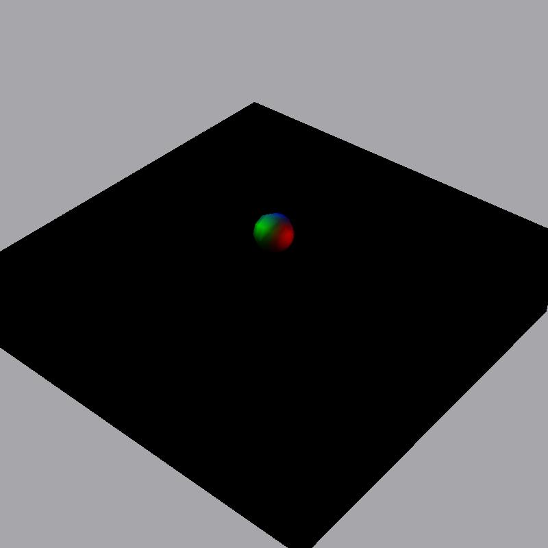
Art contest
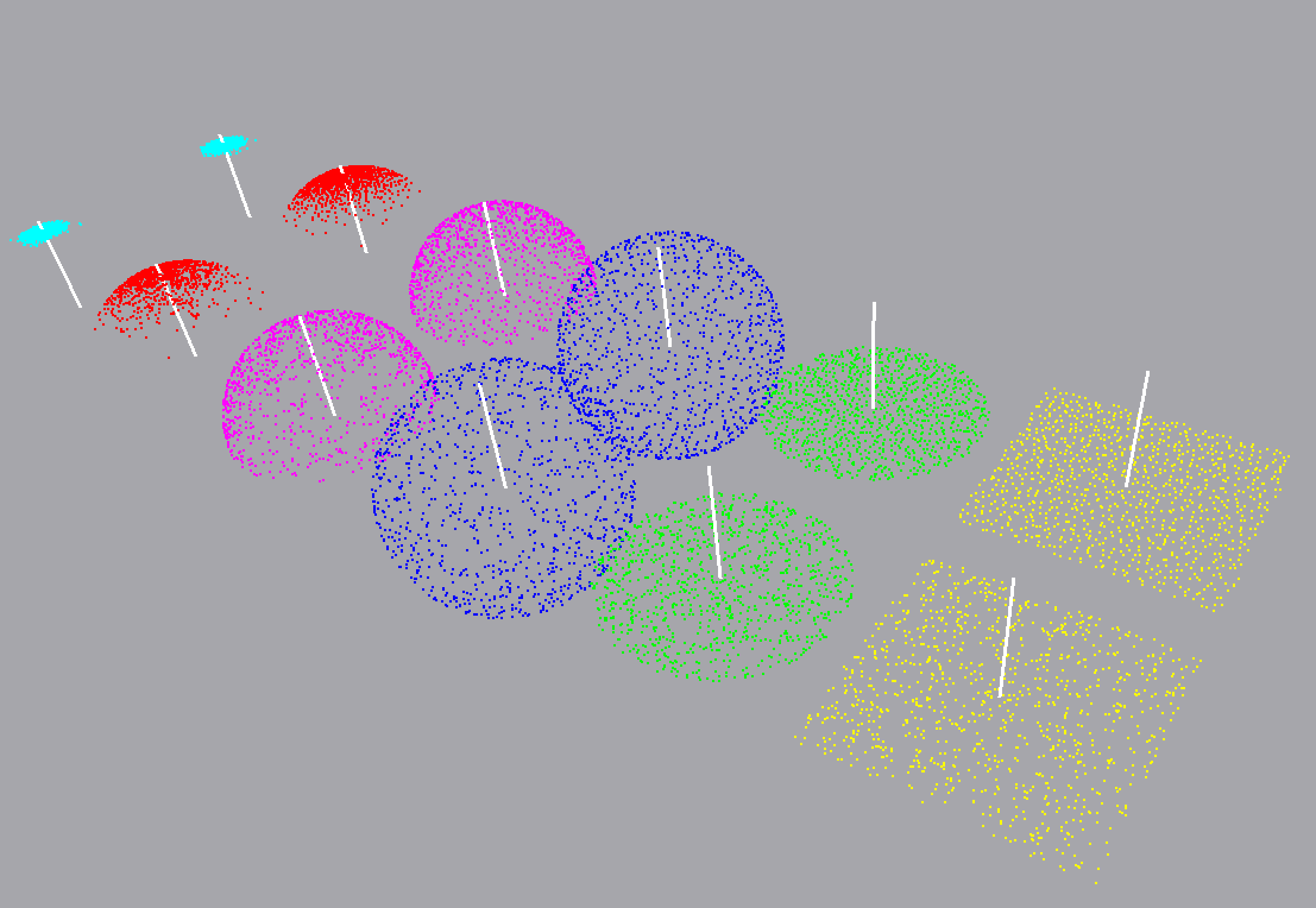
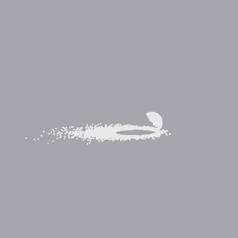
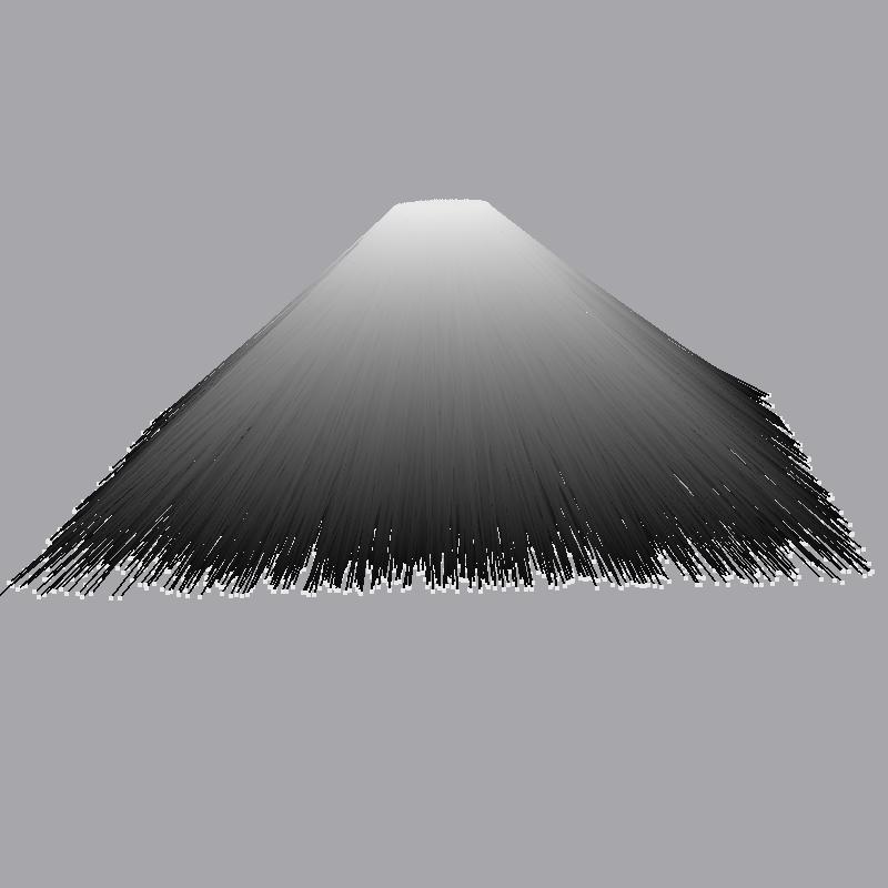
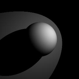
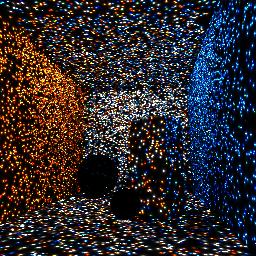
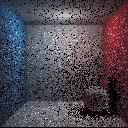
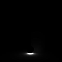
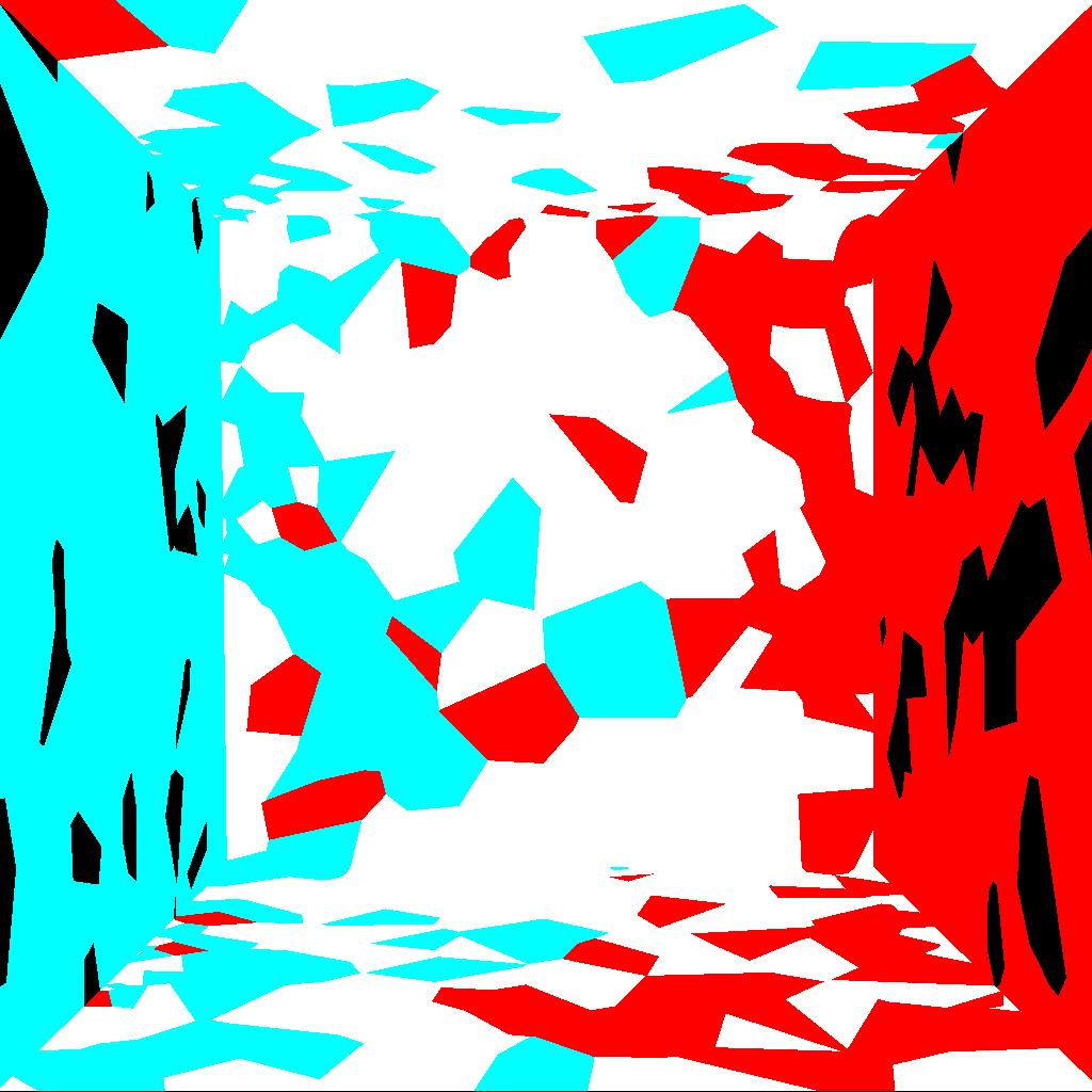
I have decided to submit an image that my program has outputted as a part of debugging process - this is estimation of global photon map. The error in normalization factor has caused the creation of this 'accidental' art, that I feel has quite pleaseing minimalistic qualities.
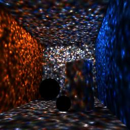
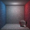
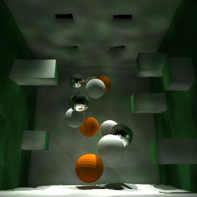
To show that I am not just giving it up cheaply I was also working on a custom scene, however sadly the meshes imported from blender are rendered faceted. I simply like above image more then the one below. I was going for sort of mysitc cave look, however I was having troubles making sure the holes in the ceiling are in fact bright, and entire image could use some parameter tweaking
References
[1] Jensen 01, Practical Guide to Global Illumination using Photon Mapping, Siggraph 2001 Course 38