COS526 Fall 2012 - Assignment 3: Photon Mapping

Edward Zhang (edwardz)

Photons

The photon data structure has the following fields: There are also two debugging fields that are used for visualization

Photon Tracing

There are several distinct steps in photon tracing.
  1. Photon Emission: First of all, we generate photons from all the light sources in the image. The number of photons is set as a command line parameter. The number of photons emitted from each light source is proportional to the light source intensity.
    Since each different light type works differently, there has to be a different photon emission step for each light type. I implemented this in the emitphotons.cpp file.
    There are several interesting things to note about photon emission. First of all, there were two common functions that were used in multiple cases: one was to generate a random point on a circle, which was simply done using rejection sampling in the unit square. The other was to generate a random vector weighted by the cosine of the angle from a direction, which was done simply by uniformly sampling points on a sphere by phi and theta
    Area lights use the above two functions to generate the position and direction, respectively. Point lights were uniformly sampled from points on a sphere by inverse sampling. Spotlight photons were sampled according to the cosine distribution function, as above.
    Directional lights cause a bit of a headache because the effective power (relative to other lights) is dependent on the scene geometry. I did not choose to deal with this in any special way; powers were just set to be intensity divided by number of photons, just as for other lights. Photon positions were simply generated by generating a plane outside the bounding box of the scene. This plane was chosen to be perpendicular to the direction and tangent to the appropriate corner of the bounding box. Then, each other corner on the bounding box was projected onto the plane and points were uniformly sampled in the bounding circle of those projections.
  2. Photon Scattering, BRDF Importance Sampling, and Russian Roulette There are two utility functions used in scattering and russian roulette. The first is a RotateToVector function, which is used in BRDF Importance Sampling. This function takes a vector that is generated according to some distribution relative to the x-axis vector, and then transforms it so that it is relative to some other vector.
    The other utility function actually performs scattering and russian roulette, and is also used by the raytracing renderer. This Trace function first calculates the appropriate diffuse, specular, and transmissive powers and probabilities, according to Jensen01. Then, it randomly determines whether to reflect the incoming light (photon or ray) in a transmissive, specular, or diffuse manner according to these probabilities. I assumed that refracted rays would always undergo perfect refraction, but specular and diffuse rays were sampled according to the BRDF as specified in Jason Lawrence's course notes. Note that this function also must move the generated position a little bit off of the intersecting surface; otherwise floating point error will often cause subsequent traces to intersect the same spot.
    To actually perform photon scattering, we iterate over all the emitted photons, determine if they intersect the scene, and call Trace on them if so to determine the appropriate values for a newly generated photon (or do not generate a photon if the photon is absorbed). The photons are recursively traced if appropriate, and the old photon stored if the intersecting material is diffuse.
    A significant downside of the provided scene files is that materials do not necessarily conform to the conservation of energy constraint that the sum of the specular, diffuse, and transmissive coefficients are less than one. This causes significant problems for russian roulette, since a trace would never terminate. Therefore, I included a parameter to the Trace function that specifies an absorption probability (default 0.05). By scaling the diffuse, transmissive, and specular coefficients appropriately, this ensured that the trace would eventually terminate.

    This is a visualization of the russian roulette process in the still life scene. Notice that one path actually underwent many diffuse (cyan) and specular (magenta) reflections before terminating.
  3. Photon Storage Through the scattering process, photons are continually added to an array when they are stored. There are two arrays used; one for the global map and one for the caustic map. These arrays are used to construct photon map KD Trees after scattering has been completed.
  4. Multiple Photon Maps: Although the global illumination map deals with caustics fairly well, there are many cases where a supplemental caustic photon map helps a lot. My implementation allows the user to specify whether a caustic map is desired; a caustic map will emit many more photons than the global photon map emission (but will keep fewer of them). In the example below, you can see the difference in effect that the caustics make, especially directly behind the cube.
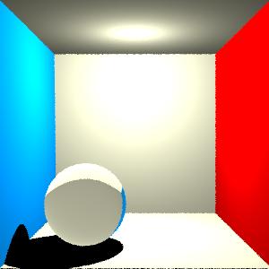
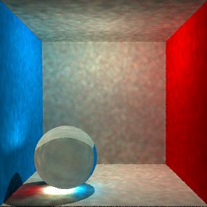
    Jello Cube with Global Illumination Photon Map Jello Cube with Caustic Photon Map and Global Map
    src/photonmap input/prism.scn output/caustic.jpg -resolution 200 200 -n 2000000 -r 500 src/photonmap input/prism.scn output/caustic.jpg -resolution 200 200 -n 2000000 -r 500 -caustic
  5. Photon Map Visualization: Since I had many odd errors earlier on, I implemented a number of ways to visualize the photons in my photon map. One that I used for large numbers of photons was a photon density map, where the intensity of each pixel was proportional to the number of photons in the map that would be projected onto that pixel. This helped me make sure photons were going where I thought they should (you can see the effect of the caustics below).
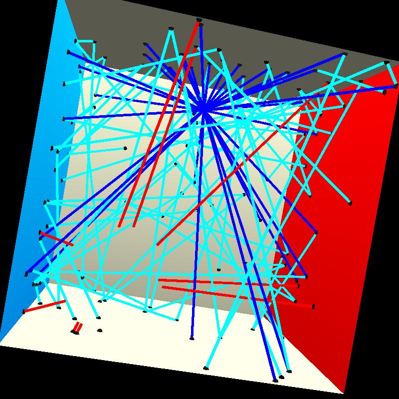
    Cornell Box Photon Density Map

    Another visualization that I used heavily visualized not only the photons, but the paths they came from. This used the optional fields in the Photon data structure, and rendered the paths using cylinders of different colors. This system is totally unusable with any more than several hundred photons, however.
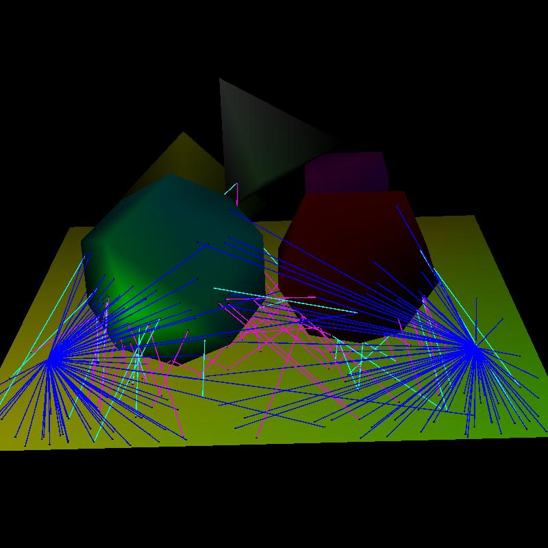
    Cornell Box Photon Visualization Still Life Photon Visualization

Radiance Estimation at a Point

Radiance estimation at a point includes three components: direct lighting, radiance from photon maps, and ray tracing. Note that the first bounce of a photon is never stored at diffuse surfaces, since that component is included in the direct lighting calculation.
Direct Lighting Only Monte Carlo Path Tracing (with russian roulette) and Direct Lighting Photon Map, Direct Lighting, and Path Tracing
500000 photons, 200 nearest photons
src/photonmap input/cornell.scn output/all.jpg -resolution 300 300 -n 500000 -r 200
50 Photon Neighborhood 200 Photon Neighborhood 500 Photon Neighborhood
We can see the results of having various photon neighborhood sizes (number of nearest neighbors) in the images above. In the caustics in the shaded region, we see a speckled pattern with fewer photons in the neighborhood (also appears in the cornell box), but with more photons in the neighborhood the caustics become much smoother.

Rendering (Camera Ray Tracing, Pixel Integration/Multisampling)

To render an entire image, I generate some number of rays within each pixel for antialiasing (default 3, which is what all images here are rendered with). Each of these rays is then tested for scene intersection, then rendered according to the radiance estimation described above. Finally, some scaling needs to be done so that pixels have valid values (0-255 RGB). Via a combination of adjusting light parameters and scaling such that pixels too far above the mean value were clamped, I managed to get acceptable results. This can actually be observed in the above set of images; note that the images without global illumination appear overall brighter, whereas the only really bright spot in the photon mapped image is the caustic under the sphere.
My scaling decision was somewhat arbitrary, but it meant that tuning lighting parameters was easier since I could see most of the range of variance in the illumination. I'd probably let more clamping happen if I were trying to go for the best appearance.

Sample Image Results

The most interesting effects obtainable with photon maps are diffuse interreflection and caustics. I created my own simple scene of a red "jello" cube on a table to look at caustic effects, and the default cornell box has a great demonstration of diffuse interreflection near the back walls.
Jello Cube showing Caustics Cornell Box showing interreflection

General Observations about the project: